Structure enumeration

In this notebook we employ structure enumeration to generate structures. Structure enumeration is a method that generates all symmetrically inequivalent structures that are permissible given a certain lattice.

The procedure was developed and is described in Physical Review B 77, 224115 (2008).

Simple example

Let us first enumerate structures based on a FCC lattice, represented by the case of Au below.

%%time
from ase.build import bulk
from icet.tools import enumerate_structures

# set up primitive structure
primitive_structure = bulk('Au')

# specify species allowed on each sublattice
chemical_symbols = ['Au', 'Pd']

# supercell sizes to consider
sizes = range(1, 10)

# run enumeration
structures = list(enumerate_structures(
    primitive_structure,
    sizes=sizes,
    chemical_symbols=chemical_symbols,
))
print(f'Number of structures:: {len(structures)}')

Number of structures:: 1135
CPU times: user 4.05 s, sys: 6.9 s, total: 11 s
Wall time: 2.17 s

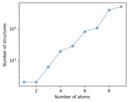
The number of distinct structures increases quickly with the number of available sites as shown by the figure below. One shoul

count_by_size = {}
for structure in structures:
    natoms = len(structure)
    count_by_size[natoms] = count_by_size.get(natoms, 0) + 1
count_by_size

{1: 2, 2: 2, 3: 6, 4: 19, 5: 28, 6: 80, 7: 104, 8: 390, 9: 504}

from matplotlib import pyplot as plt

fig, ax = plt.subplots(
    figsize=(4.5, 3.6),
    dpi=120,
)

ax.plot(count_by_size.keys(), count_by_size.values(), 'o-', alpha=0.5)

ax.set_xlabel('Number of atoms')
ax.set_ylabel('Number of structures')
ax.set_yscale('log')

fig.tight_layout()

By enumerating structures we can systematically map out the accessible cluster vector space. This allows us to illustrate some important points.

Point 1: The elements of the cluster vector cannot adopt values independently of each other.

This is as a result of the natural correlation of a structure. For example, for a given concentration (i.e., a specific value of the singlet) the values that the first nearest neighbor cluster function can adopt are limited.

Point 2: The most extreme combinations of cluster function values are typically reached in rather small cells already.

This is actually good news since it means that we can use small cells (and hence carry out less expensive calculations) when constructing a cluster expansion. Conversely larger cells with less order yield comparably less information. As an extreme case, consider special quasi-random structures (SQSs). In such a case, we try to emulate a situation where the cluster vector values assume the most average vale .

To demonstrate these points in the next cell we first compile the cluster vectors of the structures that we enumerated above.

import numpy as np
from icet import ClusterSpace

cs = ClusterSpace(primitive_structure, [8.0, 5.0], chemical_symbols)

A, natoms = [], []
for structure in structures:
    A.append(cs.get_cluster_vector(structure))
    natoms.append(len(structure))
A = np.array(A)

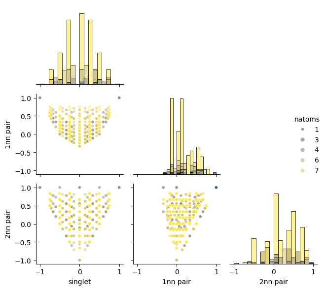
Next we plot the correlation of a few cluster function values. Here, we consider only the singlet and the first two pairs but you can easily modify the cell below to inspect the correlation of higher-order lusters as well.

The figure clearly shows that there are certain parts of the space that cannot be reached (see point 1 above). For example, if the singlet is below -0.5, we cannot generate a structure for which the first nearest neighbor pair adopts a negative value.

Moreover one can see that the boundaries of the accessible space are delineated by small structures (see point 2 above). Larger (less ordered) structures fall in between these limits.

import seaborn as sns
from pandas import DataFrame

columns = ['singlet', '1nn pair', '2nn pair']
df = DataFrame(A[:, 1:len(columns) + 1], columns=columns)
df['natoms'] = natoms
df = df[df.natoms <= 8]

g = sns.PairGrid(df, corner=True, hue='natoms', palette='cividis', height=2)
g.map_diag(sns.histplot)
g.map_offdiag(sns.scatterplot, alpha=0.5, size=1)
g.add_legend()

g.set(xlim=(-1.1, 1.1))
g.set(ylim=(-1.1, 1.1))
plt.tight_layout()

Structure enumeration with constraints

It is not unusual that one is only interested in a certain composition range. For example, for a structure containing vacancies one typically would want to limit the vacancy concentration to a certain maximum value. This can be done using concentration restrictions as illustrated for the case of \(\ce{Mo_{1-x}V_x:C_{1-y}}\) below, where \(x\) is the vanadium and \(y\) the vacancy concentration.

Note: Below “Be” is used to represent a vacant site.

from ase.io import read

# read primitive structure
prim = read('../structures/MoC_rocksalt_prim.xyz')

# specify species allowed on each sublattice
chemical_symbols = [['Mo', 'V'] if s == 'Mo' else ['C', 'Be'] for s in prim.symbols]

# supercell sizes to consider
sizes = range(1, 7)

# limit the vacancy (=Be) concentration to below 15%
concentration_restrictions = {'Be': (0, 0.15)}

# run enumeration
structures = list(enumerate_structures(
    prim, sizes=sizes, chemical_symbols=chemical_symbols,
    concentration_restrictions=concentration_restrictions))
print(f'Number of structures:: {len(structures)}')

Number of structures:: 667