Active learning
Here, we will demonstrate how one can generate a set of training structures based on active learning.
The cluster expansion (CE) is trained iteratively and new structures are selected in each iteration based on the model uncertainty prediction for a pool of structures. The uncertainty of structures can be estimated from, for example, an ensemble of CEs from bootstrap sampling.
More details regarding the approach can be found in Advanced Theory and Simulations 2, 1900015 (2019) and in Journal of Physics: Energy 3, 034012 (2021).
Ensemble of cluster expansions
First, we start from a small set of initial training structures. These training structures are split into several different training sets using boostrap sampling or sampling with replacements, and each of these training sets is used to train a CE.
Structure selection
This produces an ensemble of CEs, or an ensemble of ECIs, \(\boldsymbol{w}_i\), where \(i\) refers to \(i\)-th CE in the ensemble. For a given structure with cluster vector \(\boldsymbol{X}\) we can now predict its mean energy and its standard deviation using the ensemble as
and
where \(\boldsymbol{X} \cdot \boldsymbol{w}_i\) is the energy predicted for the structure using the \(i\)-th cluster expansion.
If all CEs in the ensemble predict (almost) the same energy for a given structure then likely this is not a good structure to add to the training set. However, if the CEs predict wildly different eneriges for a structures, i.e., small differences in the training sets lead to large differences when predicting the energy of this structures, then this is a good structure to add to the training set.
Training an ensemble of models
First, we train an ensemble of models using the EnsembleOptimizer. Here, we will read the structures from the DFT database rocksalt_MoVCvac_uncertainty.db. Note that this databases contains structures generated from 8 iterations of active learning, but here we only include structures up to the 4th generation.
Note: Below “Be” is used to represent a vacant site.
[1]:
from ase.db import connect
from ase.io import read
from icet import ClusterSpace, StructureContainer

# parameters
ensemble_size = 100
fit_method = 'ardr'
cutoffs = [9.0, 5.0]

# set up ClusterSpace and StructureContainer
prim = read('../structures/MoC_rocksalt_prim.xyz')
chemical_symbols = [['C', 'Be'], ['Mo', 'V']]
cs = ClusterSpace(prim, cutoffs, chemical_symbols)
sc = StructureContainer(cs)

# collect training structures
# we only include structures up to the fourth
# generation for the purpose of demonstration
maxgen = 4
tags_to_keep = ['initial'] + [f'gen{it}' for it in range(0, maxgen)]
db = connect('../dft-databases/rocksalt_MoVCvac_uncertainty.db')
for row in db.select():
    if any([tag_to_keep in row.tag for tag_to_keep in tags_to_keep]):
        sc.add_structure(row.toatoms(), user_tag=row.tag,
                         properties=dict(mixing_energy=row.mixing_energy))
sc
[1]:
Structure Container
Total number of structures: 102
| user_tag | natoms | formula | mixing_energy | |
|---|---|---|---|---|
| 0 | initial_it0 | 2 | MoC | 0.000000 |
| 1 | initial_it1 | 2 | VC | 0.000000 |
| 2 | initial_it2 | 12 | BeMoV5C5 | 0.081152 |
| 3 | initial_it3 | 12 | BeMoV5C5 | -0.004243 |
| 4 | initial_it4 | 8 | BeV4C3 | 0.067426 |
| ... | ... | ... | ... | ... |
| 97 | uncertainty_gen3_it17 | 128 | Be11Mo31V33C53 | -0.089592 |
| 98 | uncertainty_gen3_it1 | 128 | Be19Mo39V25C45 | -0.082065 |
| 99 | uncertainty_gen3_it8 | 128 | Be14Mo47V17C50 | -0.102671 |
| 100 | uncertainty_gen3_it13 | 128 | Be8Mo37V27C56 | -0.083576 |
| 101 | uncertainty_gen3_it9 | 54 | Be4Mo21V6C23 | -0.086451 |
102 rows × 4 columns
[2]:
from trainstation import EnsembleOptimizer

# training with EnsembleOptimizer
A, y = sc.get_fit_data(key='mixing_energy')
eopt = EnsembleOptimizer((A, y), ensemble_size=ensemble_size, fit_method=fit_method)
eopt.train()
print(eopt)
================= EnsembleOptimizer ==================
seed                           : 42
fit_method                     : ardr
standardize                    : True
n_target_values                : 102
n_parameters                   : 52
n_nonzero_parameters           : 52
parameters_norm                : 0.3737099
target_values_std              : 0.05996159
rmse_train                     : 0.004625389
rmse_test                      : 0.01243977
ensemble_size                  : 100
train_size                     : 102
bootstrap                      : True
======================================================
Generating structures with MC
Next, we generate a pool of structures by running simulated annealing MC simulations in the canonical ensemble with varyning supercell sizes and concentrations. This ensures that we sample large parts of the configurational space but also that only thermodynamically relevant structures are generated. Here, one should also keep in mind to run small supercell sizes for which DFT calculations are not too expensive.
Note that we only run a few rather short MC simulations in order for demonstration purposes, but in principle one could/should run more and longer simulations.
[3]:
%%time

import numpy as np
from icet import ClusterExpansion
from mchammer.ensembles import CanonicalAnnealing
from mchammer.calculators import ClusterExpansionCalculator

# parameters
x_vacancy_max = 0.3  # maximum carbon-vacancy concentration
supercell_sizes = [
    (2, 2, 3), (2, 3, 5), (3, 5, 7), (2, 2, 7),
    (2, 2, 8), (3, 3, 6), (3, 3, 3), (4, 4, 4),
]

# cluster expansion
ce = ClusterExpansion(cs, eopt.parameters)

# MC params
T_start = 3000
T_stop = 1
MC_cycles = 200
dump_interval = 1

# read cluster expansion
concs = []
for size in supercell_sizes:

    # generate random supercell
    supercell = prim.repeat(size)
    n_sublattice_sites = len(supercell) // 2

    n_Mo = np.random.randint(0, n_sublattice_sites + 1)
    n_V = n_sublattice_sites - n_Mo
    n_C = np.random.randint(
        int((1-x_vacancy_max) * n_sublattice_sites), n_sublattice_sites + 1)
    n_Be = n_sublattice_sites - n_C

    metal_symbols = ['Mo'] * n_Mo + ['V'] * n_V
    carbon_symbols = ['C'] * n_C + ['Be'] * n_Be
    supercell.symbols[supercell.symbols == 'Mo'] = metal_symbols
    supercell.symbols[supercell.symbols == 'C'] = carbon_symbols

    # run MC
    n_steps = MC_cycles * 2 * n_sublattice_sites
    size_tag = 'x'.join(str(s) for s in size)
    tag = f'gen{maxgen}_size{size_tag}_nMo{n_Mo}_nC{n_C}'
    dc_filename = f'data_containers/dc_{tag}.dc'
    calc = ClusterExpansionCalculator(supercell, ce)
    print(f'Running MC for {tag}')
    mc = CanonicalAnnealing(
        supercell, calc, T_start=T_start, T_stop=T_stop, n_steps=n_steps,
        dc_filename=dc_filename,
        ensemble_data_write_interval=n_sublattice_sites,
        trajectory_write_interval=n_sublattice_sites,
        cooling_function='linear')
    mc.run()
icet: WARNING  The ClusterExpansionCalculator self-interacts, which may lead to erroneous results. To avoid self-interaction, use a larger supercell or a cluster space with shorter cutoffs.
Running MC for gen4_size2x2x3_nMo8_nC9
icet: WARNING  The ClusterExpansionCalculator self-interacts, which may lead to erroneous results. To avoid self-interaction, use a larger supercell or a cluster space with shorter cutoffs.
Running MC for gen4_size2x3x5_nMo25_nC22
icet: WARNING  The ClusterExpansionCalculator self-interacts, which may lead to erroneous results. To avoid self-interaction, use a larger supercell or a cluster space with shorter cutoffs.
Running MC for gen4_size3x5x7_nMo51_nC83
icet: WARNING  The ClusterExpansionCalculator self-interacts, which may lead to erroneous results. To avoid self-interaction, use a larger supercell or a cluster space with shorter cutoffs.
Running MC for gen4_size2x2x7_nMo27_nC27
icet: WARNING  The ClusterExpansionCalculator self-interacts, which may lead to erroneous results. To avoid self-interaction, use a larger supercell or a cluster space with shorter cutoffs.
Running MC for gen4_size2x2x8_nMo16_nC27
icet: WARNING  The ClusterExpansionCalculator self-interacts, which may lead to erroneous results. To avoid self-interaction, use a larger supercell or a cluster space with shorter cutoffs.
Running MC for gen4_size3x3x6_nMo31_nC46
icet: WARNING  The ClusterExpansionCalculator self-interacts, which may lead to erroneous results. To avoid self-interaction, use a larger supercell or a cluster space with shorter cutoffs.
Running MC for gen4_size3x3x3_nMo12_nC19
icet: WARNING  The ClusterExpansionCalculator self-interacts, which may lead to erroneous results. To avoid self-interaction, use a larger supercell or a cluster space with shorter cutoffs.
Running MC for gen4_size4x4x4_nMo4_nC51
CPU times: user 37.5 s, sys: 4.51 s, total: 42 s
Wall time: 36.4 s
Selecting structures based on uncertainty
The MC simulations above produce a number of DataContainers that contain the trajectories of each simulation. Next, we evaluate the energy uncertainty along these trajectories and select the snapshot with highest uncertainty from each simulation.
[4]:
%%time
import glob
import pandas as pd
from mchammer import DataContainer

selected_snapshots = []
for dc_fname in sorted(glob.glob('data_containers/*.dc')):

    # read DataContainer
    dc = DataContainer.read(dc_fname)
    traj = dc.get('trajectory')

    # compute uncertainty along the trajectory
    records = []
    for iframe, structure in enumerate(traj):

        # get uncertainty
        # Here, we compute the energies by directly dotting the cluster
        # vector with the ECIs to avoid recomputing the cluster vector
        # with each CE (and thus saving time).
        cv = cs.get_cluster_vector(structure)
        energies = np.dot(eopt.parameters_splits, cv)

        # compile results
        records.append(dict(
            iframe=iframe,
            energy_mean=np.mean(energies),
            energy_std=np.std(energies),
        ))

    df = pd.DataFrame(records)

    # select structure with largest uncertainty
    ind = df.energy_std.idxmax()
    structure = traj[ind]
    selected_snapshots.append(structure)
    print(f'{dc_fname.split("/")[-1]:36}  selected index= {ind:3}'
          f'   energy_std= {1e3 * df.energy_std.max():.2f} meV/atom')
dc_gen4_size2x2x3_nMo10_nC8.dc        selected index=  31   energy_std= 9.43 meV/atom
dc_gen4_size2x2x3_nMo1_nC9.dc         selected index=  30   energy_std= 7.19 meV/atom
dc_gen4_size2x2x3_nMo8_nC9.dc         selected index=  14   energy_std= 7.40 meV/atom
dc_gen4_size2x2x3_nMo9_nC11.dc        selected index= 110   energy_std= 5.93 meV/atom
dc_gen4_size2x2x7_nMo27_nC27.dc       selected index=   0   energy_std= 6.18 meV/atom
dc_gen4_size2x2x7_nMo4_nC23.dc        selected index=  40   energy_std= 5.01 meV/atom
dc_gen4_size2x2x7_nMo6_nC19.dc        selected index=  88   energy_std= 8.62 meV/atom
dc_gen4_size2x2x7_nMo6_nC26.dc        selected index=  93   energy_std= 4.34 meV/atom
dc_gen4_size2x2x8_nMo13_nC25.dc       selected index= 292   energy_std= 5.64 meV/atom
dc_gen4_size2x2x8_nMo16_nC27.dc       selected index= 348   energy_std= 6.07 meV/atom
dc_gen4_size2x2x8_nMo1_nC29.dc        selected index= 130   energy_std= 3.89 meV/atom
dc_gen4_size2x2x8_nMo25_nC28.dc       selected index= 199   energy_std= 6.14 meV/atom
dc_gen4_size2x3x5_nMo0_nC27.dc        selected index= 100   energy_std= 4.55 meV/atom
dc_gen4_size2x3x5_nMo15_nC21.dc       selected index= 267   energy_std= 8.31 meV/atom
dc_gen4_size2x3x5_nMo25_nC22.dc       selected index=   0   energy_std= 6.59 meV/atom
dc_gen4_size2x3x5_nMo5_nC30.dc        selected index= 384   energy_std= 4.38 meV/atom
dc_gen4_size3x3x3_nMo11_nC26.dc       selected index= 316   energy_std= 7.18 meV/atom
dc_gen4_size3x3x3_nMo12_nC19.dc       selected index=  62   energy_std= 9.82 meV/atom
dc_gen4_size3x3x3_nMo25_nC24.dc       selected index=  87   energy_std= 5.84 meV/atom
dc_gen4_size3x3x3_nMo27_nC19.dc       selected index= 122   energy_std= 8.11 meV/atom
dc_gen4_size3x3x6_nMo20_nC43.dc       selected index= 196   energy_std= 7.04 meV/atom
dc_gen4_size3x3x6_nMo31_nC46.dc       selected index= 340   energy_std= 6.84 meV/atom
dc_gen4_size3x3x6_nMo3_nC49.dc        selected index= 231   energy_std= 3.78 meV/atom
dc_gen4_size3x3x6_nMo49_nC45.dc       selected index= 379   energy_std= 6.30 meV/atom
dc_gen4_size3x5x7_nMo102_nC76.dc      selected index= 251   energy_std= 5.87 meV/atom
dc_gen4_size3x5x7_nMo23_nC100.dc      selected index= 388   energy_std= 5.75 meV/atom
dc_gen4_size3x5x7_nMo40_nC87.dc       selected index= 357   energy_std= 6.16 meV/atom
dc_gen4_size3x5x7_nMo51_nC83.dc       selected index= 318   energy_std= 5.72 meV/atom
dc_gen4_size4x4x4_nMo38_nC58.dc       selected index= 396   energy_std= 6.26 meV/atom
dc_gen4_size4x4x4_nMo49_nC62.dc       selected index= 396   energy_std= 4.89 meV/atom
dc_gen4_size4x4x4_nMo4_nC51.dc        selected index=  74   energy_std= 5.70 meV/atom
dc_gen4_size4x4x4_nMo9_nC56.dc        selected index= 361   energy_std= 5.25 meV/atom
CPU times: user 3min 6s, sys: 1.11 ms, total: 3min 6s
Wall time: 6min 9s
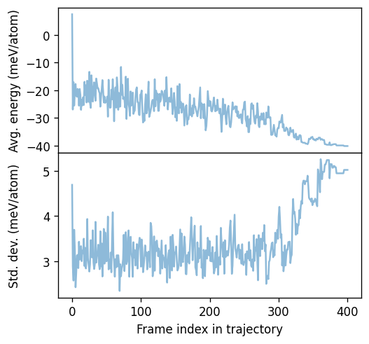
The list selected_snapshots now contains the new structures to be added to the training set.
For illustration we can also plot the uncertainty along a MC simulation.
[5]:
from matplotlib import pyplot as plt

fig, axes = plt.subplots(
    figsize=(4.5, 4.2),
    dpi=120,
    nrows=2,
    sharex=True,
)

ax = axes[0]
ax.plot(df.iframe, 1e3 * df.energy_mean, alpha=0.5, ms=2)
ax.set_ylabel('Avg. energy (meV/atom)')

ax = axes[1]
ax.plot(df.iframe, 1e3 * df.energy_std, alpha=0.5, ms=2)
ax.set_ylabel('Std. dev. (meV/atom)')
ax.set_xlabel('Frame index in trajectory')

fig.tight_layout()
fig.subplots_adjust(hspace=0)
fig.align_ylabels()