The VCSCG variance constraint \(\bar{\kappa}\)
The VCSGC ensemble requires one to specify both an average and a variance constraint for the concentration via the \(\bar{\phi}\) and \(\bar{\kappa}\) parameters. In the previous part of this tutorial we have used a value of \(\bar{\kappa}=50\). This is an optimized value for the \(\ce{Ag_{1-x}Pd_x}\) system under study here, as will be shown below. The default value suggested in the mchammer module of icet is \(\bar{\kappa}=200\), which is a more conservative choice
that works for many systems at a slight reduction in sampling efficiency as weill become apparent through the following analysis. For the majority of use cases, \(\bar{\kappa}\) can in fact be chosen over a rather wide range as shown in Physical Review B 86, 134204 (2012) and Physical Review B 85, 184203 (2012).
The present notebook explores this aspect in more detail and motivatives the above statements. The key observations are
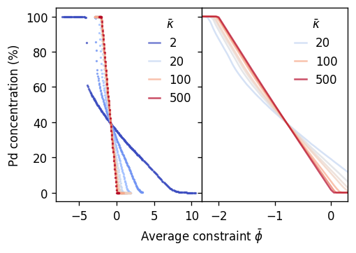
In VCSGC-MC simulations one obtains a nearly linear mapping between the average constraint parameter \(\bar{\phi}\) and the average concentration \(\left<c\right>\). VCSGC-MC simulations thus yield a more even sampling of the concentration range than SGC-MC simulations.
When increasing \(\bar{\kappa}\), the concentration range sampled for a fixed range of \(\bar{\phi}\) increases. When \(\bar{\kappa}\) approaches zero on the other hand, the VCSGC ensemble maps back to the SGC ensemble.
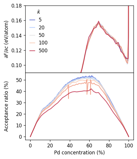
The free energy derivative is independent of the choice of \(\bar{\kappa}\).
The acceptance ratio drops, however, with increasing \(\bar{\kappa}\), which means that longer runs are needed to achieve convergence. This is also evident from the statistical error of the free energy estimate, which increases with \(\bar{\kappa}\).
Load data
Below we first define a function for parsing DataContainer files and collecting averages. This function is almost identical to the function defined in the SGC-VCGSGC analysis notebook.
[1]:
import numpy as np
from glob import glob
from mchammer import DataContainer
from pandas import DataFrame
try:
    from tqdm import tqdm
except ImportError:
    # Make the collect_averages function work even if you do not have tqdm installed.
    def tqdm(arg): return arg

def collect_averages(files: list[str], nequil: int) -> DataFrame:
    """This function loops over the list of data container file names,
    computes averages and error estimates, and returns the results in
    the form of a DataFrame.

    Parameters
    ----------
    files
        List of file names of DataContainers.
    nequil
        Number of MC cycles to drop from the beginning of the
        trajectory in order to account for equilibration.
    """

    # suppress RuntimeWarnings due to division by zero
    # Division by zero occur when computing standard deviations and
    # errors over data series with no variation. Since this is
    # inconsequential for the present purpose we turn off the warnings.
    np.seterr(invalid='ignore')

    # loop over DataContainer files
    data = []
    for fname in tqdm(files):
        dc = DataContainer.read(fname)

        # compile basic run parameters
        n_sites = dc.ensemble_parameters['n_atoms']
        record = dict(
            ensemble=dc.metadata['ensemble_name'],
            temperature=dc.ensemble_parameters['temperature'],
            n_sites=n_sites,
            n_samples=len(dc.data),
        )
        if 'vcsgc' in fname:
            record['phi'] = dc.ensemble_parameters['phi_Pd']
            record['kappa'] = dc.ensemble_parameters['kappa']
        else:
            record['dmu'] = dc.ensemble_parameters['mu_Pd']
        data.append(record)

        # compute averages for several properties
        properties = ['potential', 'Pd_count', 'acceptance_ratio']
        for p in ['sro_Ag_1', 'free_energy_derivative_Pd']:
            if p in dc.data:
                properties.append(p)
        for prop in properties:
            # drop the first nequil MC cycles for equilibration
            result = dc.analyze_data(prop, start=nequil * n_sites)
            record.update({f'{prop}_{key}': value for key, value in result.items()})

    # convert list of dicts to DataFrame
    results = DataFrame.from_dict(data)

    # ... and normalize several quantities by number of sites (or atoms)
    for fld in ['mean', 'std', 'error_estimate']:
        results[f'potential_{fld}'] /= results.n_sites
        results[f'conc_{fld}'] = results[f'Pd_count_{fld}'] / results.n_sites

    return results
Next we use the collect-averages function to compile the results. Specifically we analyze a set VCSGC-MC simulations that were run for a range of values of \(\bar{\kappa}\) at a single temperature (300 K). You can easily carry out these simulations yourself and/or more cases by modifying the run-vcsgc-simulations.py script.
[2]:
files = sorted(glob('runs-vcsgc-kappa*/vcsgc-*T300*.dc'))
results_vcsgc = collect_averages(files, nequil=10)
100%|██████████| 1159/1159 [01:23<00:00, 13.87it/s]
Variation of concentration with \(\bar{\phi}\)
We can now plot the average concentration observed during a run as a function of the average constraint parameter \(\bar{\phi}\) for several different values of \(\bar{\kappa}\).
One observes that if the variance constraint is \(\bar{\kappa}\gtrsim 50\), one obtains a practically linear mapping between \(\bar{\phi}\) and \(\langle c\rangle\) according to \(\left<c\right> \approx - \bar{\phi} / 2\). The origin of this relationship is discussed in Sec. IV.B of the tutorial paper.
This linear relationship and its weak dependence on \(\bar{\kappa}\) allows one to 1. achieve an equidistant (even) sampling of the composition range by choosing equidistant values of \(\bar{\phi}\) and 1. implies that the range over which \(\bar{\phi}\) needs to be varied in order to sample the full composition range is \(-2-\delta \lesssim \bar{\phi} \lesssim \delta\) for most use cases. Empirically one finds that \(\delta\approx 0.3\) is usually a safe choice.
As \(\bar{\kappa}\) decreases the relation between \(\bar{\phi}\) and \(\langle c\rangle\) becomes increasingly nonlinear and for the smallest values one observes that some concentrations on the Ag-rich side region can no longer be sampled. This concentration ranges corresponds to the miscibility gap. This observation is consistent with the VCSGC ensemble converging to the SGC ensemble in the limit \(\bar{\kappa}\rightarrow 0\), as the SGC ensemble cannot access two-phase regions (miscibility gaps).
[3]:
from matplotlib import pyplot as plt, colormaps

fig, axes = plt.subplots(
    figsize=(4.5, 3),
    dpi=120,
    ncols=2,
    sharey=True,
)

cmap = colormaps['coolwarm']

log_kappa_min = np.log(results_vcsgc.kappa.min())
log_kappa_max = np.log(results_vcsgc.kappa.max())

for kappa, df in results_vcsgc.groupby('kappa'):
    df.sort_values('phi', inplace=True)
    color = cmap((np.log(kappa) - log_kappa_min) / (log_kappa_max - log_kappa_min))
    label = f'{kappa}' if kappa in [2, 20, 100, 500] else ''
    kwargs = dict(alpha=0.7, color=color)
    axes[0].scatter(df.phi, 1e2 * df.conc_mean, s=1, **kwargs)
    axes[0].plot(np.nan, np.nan, label=label, **kwargs)
    if kappa >= 20:
        axes[1].plot(df.phi, 1e2 * df.conc_mean, label=label, **kwargs)

ax = axes[0]
ax.set_xlabel(r'Average constraint $\bar{\phi}$', x=1)
ax.set_ylabel(r'Pd concentration (%)')
ax.legend(title=r'$\bar{\kappa}$', handlelength=1, frameon=False)

ax = axes[1]
ax.legend(title=r'$\bar{\kappa}$', handlelength=1, frameon=False)
ax.set_xlim(-2.3, 0.3)

fig.subplots_adjust(wspace=0)

Free energies and acceptance ratios
Next we consider the free energy derivative and the acceptance ratio.
The figure below confirms that (as expected) the free energy derivative obtained from the VCSGC-MC simulations is independent of the choice of \(\bar{\kappa}\). One notes, however, that the acceptance ratio decreases as \(\bar{\kappa}\) increases. This aspect is analyzed more closely in the next cell.
[4]:
from matplotlib import pyplot as plt, colormaps

fig, axes = plt.subplots(
    figsize=(4, 5),
    dpi=120,
    nrows=2,
    sharex=True,
)

cmap = colormaps['coolwarm']

kappa_min = 5

log_kappa_min = np.log(kappa_min)
log_kappa_max = np.log(results_vcsgc.kappa.max())

for kappa, df in results_vcsgc.groupby('kappa'):
    if kappa < kappa_min:
        continue
    df.sort_values('phi', inplace=True)
    kwargs = dict(
        alpha=0.7,
        label=f'{kappa}' if kappa in [5, 20, 50, 100, 500] else '',
        color=cmap((np.log(kappa) - log_kappa_min) / (log_kappa_max - log_kappa_min)),
    )
    axes[0].plot(1e2 * df.conc_mean, df.free_energy_derivative_Pd_mean, **kwargs)
    axes[1].plot(1e2 * df.conc_mean, 1e2 * df.acceptance_ratio_mean, **kwargs)

axes[-1].set_xlabel(r'Pd concentration (%)')
axes[0].set_ylabel(r'$\partial F/\partial c$ (eV/atom)')
axes[1].set_ylabel(r'Acceptance ratio (%)')
axes[0].legend(title=r'$\bar{\kappa}$', handlelength=1, frameon=False)

axes[0].set_ylim(0.09, 0.18)

fig.align_ylabels()
fig.subplots_adjust(hspace=0)

Convergence considerations
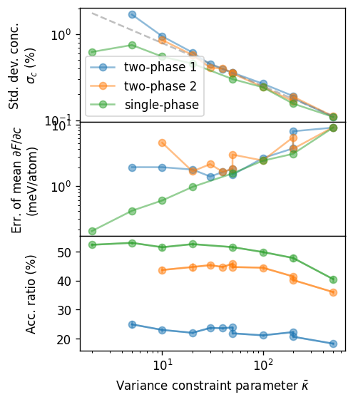
To elucidate the impact of the variance constraint parameter \(\bar{\kappa}\) on the convergence behavior of VCGSC-MC simulations we now plot explicitly plot the dependence of the standard deviation of the concentration (top panel), the error of mean of the free energy derivative (middle panel), and the acceptance ratio (bottom panel). We do this for different concentration range approximately representing one and two-phase regions, where for the latter we consider both a wider range from 1 to 86.5% and a more narrow one from 1.5 to 72.6%.
The results show that the standard deviation of the concentration drops as approximately \(\sigma_c\propto 1/\sqrt{\bar{\kappa}}\) for large \(\bar{\kappa}\) as expected given that the parameter imposes a constraint on the variance. At the same time the error of mean of the free energy derivative increases (middle panel) which is related to the decreasing acceptance ratio (lower).
One can see that the value of \(\bar{\kappa}=50\) used in the VCSGC production runs analyzed in the SGC-VCGSGC analysis notebook corresponds to a minimum in the error of mean of the free energy derivative. In general the exact location of this minimum depends on the temperature and the system. At lower temperatures and/or for systems with more pronounced miscibility gaps the minimum shifts to the larger values of \(\bar{\kappa}\). This motivates the more
conservative value of \(\bar{\kappa}=200\) used as default in the mchammer module of icet. In the present case, it leads to a higher error of mean of the free energy derivative (for a fixed number of MC steps) and hence requires more sampling to be reducded. It will, however, also perform well under more general circumstances.
[5]:
fig, axes = plt.subplots(
    figsize=(4, 5.2),
    dpi=120,
    nrows=3,
    sharex=True,
)

for k, (label, target_conc, tol) in enumerate([
        ('two-phase 1', 0.865, 0.01),
        ('two-phase 2', 0.726, 0.015),
        ('single-phase', 0.597, 0.004),
    ]):
    df = results_vcsgc[
        np.isclose(results_vcsgc.conc_mean, target_conc, atol=tol)].sort_values('kappa')
    df = df[df.kappa <= 500]

    kwargs = dict(
        color=f'C{k}',
        alpha=0.5,
        label=label,
    )

    ax = axes[0]
    ax.plot(df.kappa, 1e2 * df.conc_std, 'o-', **kwargs)
    ax.set_ylabel('Std. dev. conc.\n' + r'$\sigma_c$ (%)')

    ax = axes[1]
    ax.plot(df.kappa, 1e3 * df.free_energy_derivative_Pd_error_estimate, 'o-', **kwargs)
    ax.set_ylabel(r'Err. of mean $\partial F/\partial c$' + '\n(meV/atom)')

    ax = axes[2]
    ax.plot(df.kappa, 1e2 * df.acceptance_ratio_mean, 'o-', **kwargs)
    ax.errorbar(df.kappa, 1e2 * df.acceptance_ratio_mean,
                yerr=1e2 * df.acceptance_ratio_error_estimate, **kwargs)
    ax.set_ylabel(r'Acc. ratio (%)')

ax = axes[0]
ax.plot(df.kappa, 2.5 / df.kappa ** 0.5, '--', alpha=0.5, color='0.5')
ax.set_xscale('log')
ax.set_yscale('log')
ax.legend()

ax = axes[1]
ax.set_yscale('log')

ax = axes[-1]
ax.set_xlabel(r'Variance constraint parameter $\bar{\kappa}$')

fig.align_ylabels()
fig.subplots_adjust(hspace=0)
