SGC and VCSGC ensembles

This tutorial demonstrates how to use Monte Carlo (MC) simulations to sample the semi-grandcanonical (SGC) and variance-constained semi-grandcanonical (VCSGC) ensembles. These ensembles enable one to access the relation between composition and the first derivative of the free energy with respect to composition. While the SGC ensemble is limited to single-phase regions, the VCSGC ensemble can also be used to sample muti-phase regions.

Here, we demonstrate how to use MC simulations in these two ensembles to obtain the free energy as a function of composition and use this information to construct the phase diagram of a binary alloy. To this end, we consider the Ag-Pd system, which exhibits an asymmetric miscibility gap using a cluster expansion model from the literature (Advanced Theory and Simulations 2, 1900015 (2019)).

Background

SGC ensemble

In the case of SGC the control parameter is the chemical potential difference \(\Delta \mu_i\) of species \(i\), which for a single phase is identical to the first derivative of the free energy difference with respect to concentration,

\[\frac{1}{N} \frac{\partial \Delta F}{\partial c_i} = -\Delta \mu_i.\]

Here, we emphasize that these are chemical potential and free energy differences, where the difference is taken relative to one arbitrarily chosen reference species. This is a consequence of the total number of sites still being constant (hence the term “semi” in the name of the ensemble) as opposed to the grandcanonical ensemble, in which one controls the chemical potentials \(\mu_i\) and the total number of sites is allowed to fluctuate. In practice the “difference” distinction is often dropped.

VCSGC ensemble

In multi-phase regions (i.e., miscibility gaps) the mapping bewteen the free energy derivative and the composition becomes one-to-many. The SGC ensemble is therefore not able to sample systems inside such regions. To overcome this limitation the VCSGC ensemble introduce an additional constraint on the variance of the composition. There are now two control parameters, \(\bar{\phi}\) constrains the average concentration while \(\bar{\kappa}\) constrains the variance of the concentration. \(\bar{\phi}\) is equivalent to \(\Delta\mu\) in the SGC ensemble. The commonly used expression for the VCSGC potential is written such that \(\bar{\phi}\) is dimensionless, which has the added benefit of removing the need to adjust the sampling range when changing the temperature. When using implementation in the mchammer module of icet, one can therefore usually simply vary \(\bar{\phi}\) from about \(-2.3\) to about \(+0.3\) to sample the full composition range regardless of system or temperature.

In the VCSGC ensemble the free energy derivative can be computed from the average concentration \(\left<c\right>\) according to

\[\frac{1}{N}\frac{\partial F}{\partial c} = - 2k_BT\bar{\kappa}\left( \left<c\right> + \bar{\phi} / 2 \right).\]

Running simulations

Running MC simulations can take some time and commonly involves sampling over a range of temperatures and compositions. We therefore recommend to carry out these runs via regular python scripts (as opposed to running them in a notebook). The scripts for running the MC simulations for the present case can be found here (SGC) and here (VCSGC). For convenience (and to avoid unnecessary repetition) the results of the MC simulations are available for download (see below). We will use these data for the detailed analysis that follows further below. In the next section, we first illustrate the keys steps involved in setting up, running, and analyzing MC simulations in the SGC or VCSGC ensembles.

Illustrating example

Load cluster expansion

We start by loading the cluster expansion (CE). One can show a short overview of the CE by printing the object. This can be achieved via print(ce). In jupyter notebooks one can also obtain an HTML formatted version via the display command, which is implied if the variable is stated on the last line of a cell (as done here).

from icet import ClusterExpansion

ce = ClusterExpansion.read('AgPd.ce')
ce

Cluster Expansion

Field	Value
Space group	Fm-3m (225)
Sublattice A	('Ag', 'Pd')
Cutoffs	[13.0, 6.5, 6.0]
Total number of parameters (nonzero)	81 (44)
Number of parameters of order 0 (nonzero)	1 (1)
Number of parameters of order 1 (nonzero)	1 (1)
Number of parameters of order 2 (nonzero)	24 (13)
Number of parameters of order 3 (nonzero)	20 (13)
Number of parameters of order 4 (nonzero)	35 (16)
fractional_position_tolerance	2e-06
position_tolerance	1e-05
symprec	1e-05

Prepare structure

Next we set up supercell structure for the simulation. The primitive structure is based on an FCC lattice. To maximize the spacing between equivalent sites (and also for ease of visualization) it is preferable to use a conventional (simple cubic) cell. We therefore first convert the FCC lattice to the conventional cell before repeating the cell, where size specifies the number of unit cells in each direction.

We can obtain an abbreviated view of the structure (an ase.Atoms object) by stating the variable on the last line of the cell, using the same implied display mechanism as above.

import numpy as np
from ase.build import make_supercell

conventional_structure = make_supercell(
    ce.primitive_structure, [[-1, 1, 1], [1, -1, 1], [1, 1, -1]])

size = 4  # number of unit cells per direction
supercell = conventional_structure.repeat(size)
supercell

Atoms(symbols='Ag256', pbc=True, cell=[16.36, 16.36, 16.36])

Set up a cluster expansion calculator

During a MC simulation one needs to evaluate the underlying cluster expansion many times. In order to do this in a computationally efficient manner, in icet one uses a calculator object that is specific for a particular supercell. Here, we therefore set up such a calculator.

We get a warning that the calculator is self-interacting. This happens if the longest cutoff of the cluster expansion is larger than half of the shortest distance between periodic images. Here we are using a cluster expansion that was set up with very long cutoffs (13 Å for pairs). In general you should heed this warning and increase your supercell (or use shorter cutoffs when constructing the cluster expansion). Here we accept this warning for the sake of computational efficiency in this demonstration, and also because inspection of the effective cluster interactions (ECIs) shows that their values at those long distances are extremely small.

Tip: You can inspect ce.orbits_as_dataframe and plot the pair ECIs vs cluster size to confirm this for yourself.

from mchammer.calculators import ClusterExpansionCalculator

calculator = ClusterExpansionCalculator(supercell, ce)

icet: WARNING  The ClusterExpansionCalculator self-interacts, which may lead to erroneous results. To avoid self-interaction, use a larger supercell or a cluster space with shorter cutoffs.

Set up the SGC ensemble object

The next step is to configure an ensemble object, which is then used to run the MC simulation. By default the interval at which data is saved equals the number of sites in the supercell, which is a sensible choice for production runs. Here, we shorten this interval in order to also demonstrate the equilibration period.

from mchammer.ensembles import SemiGrandCanonicalEnsemble

temperature = 300  # temperature in K at which to run the simulation
dmu = 0.0  # chemical potential difference in eV/atom

mc = SemiGrandCanonicalEnsemble(
    supercell,
    calculator=calculator,
    temperature=temperature,
    chemical_potentials={'Ag': 0, 'Pd': dmu},
)

Run the SGC simulation

We are now ready to launch the simulation. Here, we run \(N_\mathrm{cycles}\) MC cycles, corresponding to \(N_\mathrm{cycles} \times N_\mathrm{sites}\) MC trials, where \(N_\mathrm{sites}\) is the number of Ag and Pd sites. For the purpose of this demonstration we only run for a small number of MC cycles. In production larger value are recommended. Generally speaking the smaller the acceptance ratio the more MC cycles are needed for convergence.

%%time
n_sites = len(supercell)
mc_cycles = 20
mc.run(n_sites * mc_cycles)

CPU times: user 1.74 s, sys: 1.11 ms, total: 1.74 s
Wall time: 1.74 s

Analyzing a simulation

The results of a MC simulation are available in the form of a data container object.

dc = mc.data_container
dc

Data Container

Field	Value
Type	DataContainer
mu_Ag	0
mu_Pd	0.0
n_atoms	256
temperature	300
date_created	2024-10-05T17:35:37
ensemble_name	SemiGrandCanonicalEnsemble
hostname	pieweack
icet_version	3.0
seed	9784498219251046
user_tag	None
username	erhart
Number of rows in data	21

Using this object we can readily analyze various properties of interest. We can for example plot the energy as well as other observables as a function of MC trial step. These data are provided in the form of a DataFrame via the data property.

dc.data

	mctrial	potential	acceptance_ratio	Ag_count	Pd_count
0	0	1.060517	0.000000	256	0
1	256	-14.002508	0.667969	155	101
2	512	-14.090610	0.453125	149	107
3	768	-14.354411	0.468750	153	103
4	1024	-14.605399	0.496094	158	98
5	1280	-14.311612	0.433594	157	99
6	1536	-14.217161	0.468750	153	103
7	1792	-14.406487	0.488281	150	106
8	2048	-14.089780	0.445312	148	108
9	2304	-14.186559	0.476562	152	104
10	2560	-14.313896	0.437500	156	100
11	2816	-14.349866	0.472656	153	103
12	3072	-14.104385	0.488281	150	106
13	3328	-14.313123	0.554688	156	100
14	3584	-14.333743	0.546875	158	98
15	3840	-14.093112	0.496094	149	107
16	4096	-14.219219	0.507812	159	97
17	4352	-14.196648	0.519531	154	102
18	4608	-14.458982	0.476562	158	98
19	4864	-14.487259	0.421875	154	102
20	5120	-14.380240	0.472656	157	99

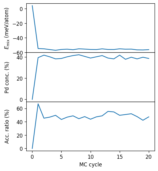
This allows us to readily plot the data. One can observe that at this temperature and chemical potential it takes about 3 to 5 MC cycles for the system to equilibrate. When computing averages we should thus exclude this part of the trajectory.

We can furthermore see that the average concentration in this simulation is about 40%. The acceptance ratio at about 50% is rather high, and we can thus expect that even relatively short runs reach convergence.

from matplotlib import pyplot as plt

fig, axes = plt.subplots(
    figsize=(4.5, 5.2),
    dpi=120,
    nrows=3,
    sharex=True,
)

ax = axes[0]
ax.plot(dc.data.mctrial / n_sites, 1e3 * dc.data.potential / n_sites)
ax.set_ylabel('$E_\mathrm{mix}$ (meV/atom)')

ax = axes[1]
ax.plot(dc.data.mctrial / n_sites, 1e2 * dc.data.Pd_count / n_sites)
ax.set_ylabel(r'Pd conc. (%)')

ax = axes[2]
ax.plot(dc.data.mctrial / n_sites, 1e2 * dc.data.acceptance_ratio)
ax.set_ylabel(r'Acc. ratio (%)')

axes[-1].set_xlabel('MC cycle')

fig.align_ylabels()
fig.subplots_adjust(hspace=0)

<>:12: SyntaxWarning: invalid escape sequence '\m'
<>:12: SyntaxWarning: invalid escape sequence '\m'
/tmp/ipykernel_119696/3580469168.py:12: SyntaxWarning: invalid escape sequence '\m'
  ax.set_ylabel('$E_\mathrm{mix}$ (meV/atom)')

Sampling the composition range

To obtain the variation of the composition with \(\Delta\mu\) and thus gain access to the mapping between the free energy derivative and the concentration, we need to run SGC-MC simulations for a range of chemical potentials. Here we pick a coarse range and also keep the relatively short simulation length that we used above, to enable short simulations suitable for this demonstration. (For the more in-depth analysis of the phase diagram that follows below, we will rely on the results from longer MC simulations for larger systems on a finer \(\Delta\mu\) grid.)

We store the results from these simulation in the form of a dictionary of DataContainer objects, which will make the analysis below straightforward.

%%time
dmus = np.linspace(-0.5, 0.3, 10)  # range of chemical potentials to sample

dcs_sgc = {}
for dmu in dmus:
    mc = SemiGrandCanonicalEnsemble(
        supercell,
        calculator=calculator,
        temperature=temperature,
        chemical_potentials={'Ag': 0, 'Pd': dmu},
    )
    mc.run(len(supercell) * mc_cycles)
    dcs_sgc[dmu] = mc.data_container

CPU times: user 13.6 s, sys: 9.67 ms, total: 13.6 s
Wall time: 13.6 s

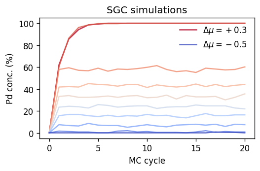
Plotting the results in the same fashion as above shows that we can access different compositions by varying \(\Delta\mu\). It also reveals that there is a range of concentrations between about 60% and 100% Pd that are not sampled after equilibration. These concentrations fall in the miscibility gap of the Ag-Pd system.

from matplotlib import colormaps

fig, ax = plt.subplots(
    figsize=(4.5, 3),
    dpi=120,
    sharex=True,
)

cmap = colormaps['coolwarm']

for dmu, dc in reversed(dcs_sgc.items()):
    n_sites = len(dc.structure)
    kwargs = dict(
        color=cmap((dmu - dmus.min()) / (dmus.max() - dmus.min())),
        label=rf'$\Delta\mu = {dmu:+.1f}$' if dmu in [dmus.max(), dmus.min()] else '',
        alpha=0.8,
    )
    ax.plot(dc.data.mctrial / n_sites,
            1e2 * dc.data.Pd_count / n_sites, **kwargs)

ax.set_title('SGC simulations')
ax.set_ylabel(r'Pd conc. (%)')
ax.set_xlabel('MC cycle')
ax.legend(frameon=False, loc='upper right')

fig.tight_layout()

Sampling with the VCSGC ensemble

As already described above, multi-phase regions (in addition to single-phase regions) can be sampled via the VCSGC ensemble. Now we therefore run a series of VCSGC-MC simulations using a similarly coarse sampling of the parameter space.

%%time
from mchammer.ensembles import VCSGCEnsemble

phis = np.linspace(-2.1, 0.1, 10)  # range of average constraint parameters to sample
kappa = 200  # a good default value

dcs_vcsgc = {}
for phi in phis:
    mc = VCSGCEnsemble(
        supercell,
        calculator=calculator,
        temperature=temperature,
        phis={'Pd': phi},
        kappa=kappa,
    )
    mc.run(len(supercell) * mc_cycles)
    dcs_vcsgc[(phi, kappa)] = mc.data_container

CPU times: user 16 s, sys: 5.17 ms, total: 16 s
Wall time: 16 s

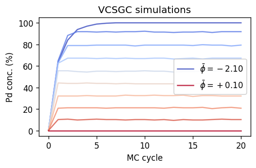
Plotting the results shows that, as expected, we can now also access concentrations inside the region between 60% and 100% Pd. One can also observe that the sampled concentrations are more evenly spaced than in the case of the SGC-MC simulations, an aspect that we will return to below.

fig, ax = plt.subplots(
    figsize=(4.5, 3),
    dpi=120,
    sharex=True,
)

cmap = colormaps['coolwarm']

for (phi, kappa), dc in dcs_vcsgc.items():
    label = r'$\bar{\phi}=' + f'{phi:+.2f}$'
    kwargs = dict(
        color=cmap((phi - phis.min()) / (phis.max() - phis.min())),
        label=label if phi in [phis.max(), phis.min()] else '',
        alpha=0.8,
    )
    ax.plot(dc.data.mctrial / n_sites,
            1e2 * dc.data.Pd_count / n_sites, **kwargs)

ax.set_title('VCSGC simulations')
ax.set_ylabel(r'Pd conc. (%)')
ax.set_xlabel('MC cycle')
ax.legend(framealpha=0.9)

fig.tight_layout()

Accessing the free energy landscape

It is now instructive to compile the results from the SGC and VCSGC-MC simulations for further comparison. To this end, we loop over the DataContainer objects generated above and use their analyze_data method. The latter allows one to readily compute mean, standard deviation, correlation time, and error estimate for a data series. From this calculation we exclude the equilibration period (given in units of MC cycles via mcc_cutoff).

from pandas import DataFrame

# suppress RuntimeWarnings due to division by zero
np.seterr(invalid='ignore')

# number of MC cycles to drop in the beginning to account for equilibration
mcc_cutoff = 5

# compile results from SGC simulations
data = []
for dmu, dc in dcs_sgc.items():
    n_sites = len(dc.structure)
    Pd_count = dc.analyze_data('Pd_count', start=mcc_cutoff * n_sites)
    data.append(dict(
        dmu=dmu,
        Pd_conc=Pd_count['mean'] / n_sites,
    ))
df_sgc = DataFrame.from_dict(data)

# compile results from VCSGC simulations
data = []
for (phi, kappa), dc in dcs_vcsgc.items():
    n_sites = len(dc.structure)
    Pd_count = dc.analyze_data('Pd_count', start=mcc_cutoff * n_sites)
    dfreen = dc.analyze_data('free_energy_derivative_Pd', start=mcc_cutoff * n_sites)
    data.append(dict(
        phi=phi,
        kappa=kappa,
        Pd_conc=Pd_count['mean'] / n_sites,
        free_energy_derivative=dfreen['mean'],
    ))
df_vcsgc = DataFrame.from_dict(data)

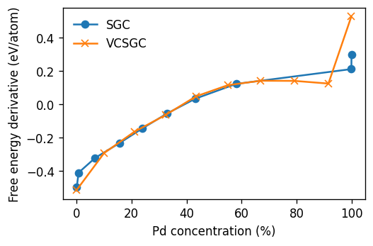
From the figure below it is apparent that in the single-phase regions, i.e., below about 60% Pd and close to 100% Pd, the SGC and VCSGC results agree. Inside the miscibility gap the mapping between the free energy derivative (from VCSGC) and the concentration is multi-valued. At these compositions the system is comprised of a region that is almost purely Pd and a region that contains about 60% Pd, separated by an interface.

Since the free energy derivative from VCSGC can be continuously mapped as a function of composition, it can be integrated to obtain the free energy. The latter contains both contributions from the bulk phases and the interface, which can also be exploited to extract interface free energies. For more information see Physical Review B 86, 134204 (2012) and Acta Materialia 227, 117697 (2022).

fig, ax = plt.subplots(
    figsize=(4.5, 3),
    dpi=120,
    sharex=True,
)

ax.plot(1e2 * df_sgc.Pd_conc, df_sgc.dmu, 'o-', label='SGC')
ax.plot(1e2 * df_vcsgc.Pd_conc, df_vcsgc.free_energy_derivative, 'x-', label='VCSGC')

ax.set_xlabel(r'Pd concentration (%)')
ax.set_ylabel('Free energy derivative (eV/atom)')
ax.legend(frameon=False)

fig.tight_layout()

Compiling the data

We will now analyze the results of the MC simulations that have been carried out using the scripts introduced in the beginning of this notebooks. We will use these data to illustrate some important aspects of SGC and VCSGC simulations, before constructing the phase diagram in the temperature-composition plane.

For convenience (and to avoid unnecessary repetition) the results of the MC simulations are available for download via zenodo and included in the underlying repository. You can find them in the form of *.dc files in the runs-* directories. We can then loop over these files and compute thermodynamic averages along with error estimates.

In the next step we do exactly that. We loop over a list of DataContainer files and use the analyze_data() method of the DataContainer object to compute the mean, standard deviation, correlation time, and error estimate (95% confidence interval) for the potential sampled in the MC simulation (i.e., the mixing energy) as well as the concentration and free energy derivative (in the case of VCSGC). Since this functionality will be reused below it is packaged into a function that is relatively long but annotated. We recommend that you read it carefully at it is meant to be adaptable to a variety use case(s).

Tip 1: The following cell takes several minutes to evaluated when using the data provided for this tutorial. We are therefore using the tqdm package to display a progress bar. This can be very useful to keep track when iterating over many instances (as in this case). If you do not have installed the tqdm (or do not want to install it), the try/except block should ensure that the function still runs as expected (except for the progress bar).

Tip 2: Pandas DataFrames can be easily written to file using the to_json() method of the DataFrame. Afterwards they can be read again using the read_json() function from the pandas module. This is very convenient, e.g., for transfering data between scripts.

from glob import glob
from mchammer import DataContainer
from pandas import DataFrame
try:
    from tqdm import tqdm
except ImportError:
    # Make the collect_averages function work even if you do not have tqdm installed.
    def tqdm(arg): return arg

def collect_averages(files: list[str], nequil: int) -> DataFrame:
    """This function loops over the list of data container file names,
    computes averages and error estimates, and returns the results in
    the form of a DataFrame.

    Parameters
    ----------
    files
        List of file names of DataContainers.
    nequil
        Number of MC cycles to drop from the beginning of the
        trajectory in order to account for equilibration.
    """

    # suppress RuntimeWarnings due to division by zero
    # Division by zero occur when computing standard deviations and
    # errors over data series with no variation. Since this is
    # inconsequential for the present purpose we turn off the warnings.
    np.seterr(invalid='ignore')

    # loop over DataContainer files
    data = []
    for fname in tqdm(files):
        dc = DataContainer.read(fname)

        # compile basic run parameters
        n_sites = dc.ensemble_parameters['n_atoms']
        record = dict(
            ensemble=dc.metadata['ensemble_name'],
            temperature=dc.ensemble_parameters['temperature'],
            n_sites=n_sites,
            n_samples=len(dc.data),
        )
        if 'vcsgc' in fname:
            record['phi'] = dc.ensemble_parameters['phi_Pd']
            record['kappa'] = dc.ensemble_parameters['kappa']
        else:
            record['dmu'] = dc.ensemble_parameters['mu_Pd']
        data.append(record)

        # compute averages for several properties
        properties = ['potential', 'Pd_count']
        for p in ['sro_Ag_1', 'free_energy_derivative_Pd']:
            if p in dc.data:
                properties.append(p)
        for prop in properties:
            # drop the first nequil MC cycles for equilibration
            result = dc.analyze_data(prop, start=nequil * n_sites)
            record.update({f'{prop}_{key}': value for key, value in result.items()})

    # convert list of dicts to DataFrame
    results = DataFrame.from_dict(data)

    # ... and normalize several quantities by number of sites (or atoms)
    for fld in ['mean', 'std', 'error_estimate']:
        results[f'potential_{fld}'] /= results.n_sites
        results[f'conc_{fld}'] = results[f'Pd_count_{fld}'] / results.n_sites

    return results

First we collect the results of the SGC simulations, dropping the first 10 (out of 100) MC cycles to allow for equilibration.

%%time
files = sorted(glob('runs-sgc/*.dc'))
results_sgc = collect_averages(files, nequil=10)

100%|██████████| 1575/1575 [01:10<00:00, 22.42it/s]

CPU times: user 1min 9s, sys: 540 ms, total: 1min 10s
Wall time: 1min 10s

Next we collect the results from the VCSGC simulations, also dropping the first 10 MC cycles. Here, we use the results obtained using a variance constraint parameter of \(\bar\kappa=50\). The role of this parameter is analyzed in a separate notebook.

%%time
files = sorted(glob('runs-vcsgc-kappa50/*.dc'))
results_vcsgc = collect_averages(files, nequil=10)

100%|██████████| 1955/1955 [02:30<00:00, 12.95it/s]

CPU times: user 2min 30s, sys: 723 ms, total: 2min 31s
Wall time: 2min 30s

Comparison between SGC and VCSGC

Before starting the analysis let us define a helper functions that splits up a dataframe into segments whenever the change in concentration between samples exceeds a threshold. This is useful to separate the different single-phase regions in the case of SGC simulations,.

def split_at_miscibility_gap(
    df: DataFrame,
    clim: float = 0.08,
) -> list[DataFrame]:
    """This function takes a DataFrame as input, checks for miscibility gaps and
    returns the single-phase regions as a list of DataFrames.

    Parameters
    ----------
    df
        Input DataFrame.
    clim
        If the change in concentration between two data points is larger than this
        value the two data points are assumed to be separated by a miscibility gap.
    """
    df.reset_index(inplace=True, drop=True)
    # Pick out the concentrations at which the spacing
    # between points changes by more than clim.
    split = df[df.conc_mean.diff() > clim]
    # Split up dataframe into segments using these concentrations
    # as boundaries.
    dfs = []
    imin = 0
    for imax in split.index:
        dfs.append(df.iloc[imin:imax])
        imin = imax
    dfs.append(df.iloc[imin:])
    return dfs

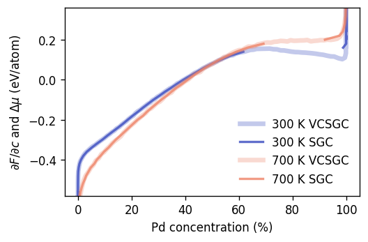
Now we plot the chemical potential (SGC) and the free energy derivative (VCSGC) as a function of the composition for two temperatures. This comparison demonstrates quantitatively the equivalence of SGC and VCSGC in single-phase regions. It moreover reveals the two-phase region in this system, which appears as a gap in the sampled composition range in SGC simulations. VCSGC simulations on the other hand allow one to access this region as well, which allows us to explicitly demonstrate the one-to-many mapping between the free energy derivative and the composition that is characteristic of this region.

# we suppress the SettingWithCopyWarning warning which appears
# when sorting the DataFrames.
import pandas as pd
pd.options.mode.chained_assignment = None  # default='warn'


fig, ax = plt.subplots(
    figsize=(4.5, 3),
    dpi=120,
    sharex=True,
    sharey=True,
)

cmap = colormaps['coolwarm']
tmin = results_vcsgc.temperature.min()
tmax = results_vcsgc.temperature.max()

for temperature in [300, 700]:
    color = cmap((temperature - tmin) / (tmax - tmin))

    # VCSGC
    df = results_vcsgc[results_vcsgc.temperature == temperature]
    df.sort_values('conc_mean', inplace=True)
    ax.plot(1e2 * df.conc_mean, df.free_energy_derivative_Pd_mean,
            label=f'{temperature:.0f} K VCSGC',
            alpha=0.3, lw=4, color=color)

    # SGC
    df = results_sgc[results_sgc.temperature == temperature]
    df.sort_values('conc_mean', inplace=True)
    label = f'{temperature:.0f} K SGC'
    for df2 in split_at_miscibility_gap(df):
        ax.plot(1e2 * df2.conc_mean, df2.dmu,
                label=label, alpha=0.8, lw=2, color=color)
        label = ''

ax.set_ylim(-0.58, 0.36)
ax.set_ylabel(r'$\partial F/\partial c$ and $\Delta\mu$ (eV/atom)')
ax.set_xlabel(r'Pd concentration (%)')
ax.legend(frameon=False)

fig.tight_layout()

VCSGC simulations

We will first take a closer look at the VCSGC results since they allow us to show the full free energy landscape and demonstrate the common tangent construction.

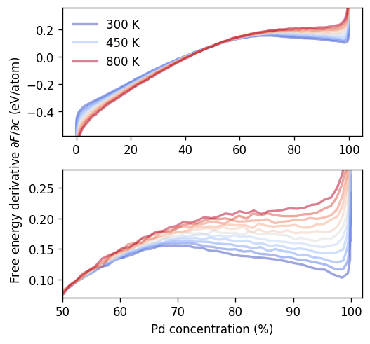
It is first instructive to consider the variation of the free energy derivative with temperature. A closer inspection of the composition range around the miscibility gap (bottom panel) shows that around 700 to 800 K the region with negative slope vanishes (in other words the minimum, maximum and inversion points coalesce), suggesting the miscibility gap closing around this temperature.

fig, axes = plt.subplots(
    figsize=(4.5, 4.2),
    dpi=120,
    nrows=2,
)

for temperature, df in results_vcsgc.groupby('temperature'):
    df.sort_values('conc_mean', inplace=True)
    color = cmap((temperature - tmin) / (tmax - tmin))
    label = f'{temperature:.0f} K' if temperature in [tmin, 450, tmax] else ''
    for ax in axes:
        ax.plot(1e2 * df.conc_mean, df.free_energy_derivative_Pd_mean,
                label=label, alpha=0.5, lw=2, color=color)

ax = axes[0]
ax.set_ylim(-0.58, 0.36)
ax.legend(frameon=False)

ax = axes[1]
ax.set_xlim(50, 102)
ax.set_ylim(0.07, 0.28)
ax.set_xlabel(r'Pd concentration (%)')
ax.set_ylabel(r'Free energy derivative $\partial F/\partial c$ (eV/atom)', y=1)

fig.tight_layout()

To obtain the phase boundaries (and thus construct the phase diagram) one can integrate the free energy derivative over composition. To this end we first define a convenience function that takes a DataFrame as input.

from scipy.integrate import cumulative_trapezoid

def compute_free_energy(results: DataFrame):
    """This function takes a DataFrame as input, and computes the free energy
    by integrating the free energy derivative obtained in VCSGC simulations.
    Data points from SGC simulations are unaffected.

    Parameters
    ----------
    results
        Input DataFrame.
    """
    for (ensemble, n_sites, temperature, kappa), df in results.groupby(
            ['ensemble', 'n_sites', 'temperature', 'kappa']):
        if ensemble != 'VCSGCEnsemble':
            continue
        df.sort_values('conc_mean', inplace=True)

        phi_min = df[df.conc_mean == 1].phi.max()
        phi_max = df[df.conc_mean == 0].phi.min()
        if phi_min is not np.nan:
            df = df[df.phi >= phi_min]
        if phi_max is not np.nan:
            df = df[df.phi <= phi_max]

        df['freen'] = 1e3 * cumulative_trapezoid(
            df.free_energy_derivative_Pd_mean, x=df.conc_mean, initial=0)
        results.loc[df.index, 'freen'] = df.freen

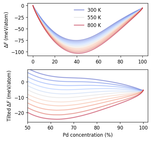
In the following cell we apply this function to our data and plot the free energy vs composition. In the upper panel, which shows the full composition range, one can observe how increasing temperatures makes mixing increasingly favorable as the mixing free energy \(\Delta F\) becomes more negative.

According to the principle of minimum free energy in equilibrium adopts the configuration corresponding to the lowest overall free energy for a given composition. In the single phase regions this is a single phase. When forced inside the miscibility gap, the system can, however, lower its energy by separating into two phases separated by an interface. The composition of the two phases as well as their relative fractions can be readily obtained via the common tangent construction and the lever rule (also compare the Maxwell construction).

To make the two-phase region more clearly visible and apply this construction, in the bottom panel the free energy landscape has been tilted by a suitably chosen constant (slope). (Note that applying a linear transformation does not affect the tangent construction.)

fig, axes = plt.subplots(
    figsize=(4.5, 4.2),
    dpi=120,
    nrows=2,
)

compute_free_energy(results_vcsgc)

for temperature, df in results_vcsgc.groupby('temperature'):
    color = cmap((temperature - tmin) / (tmax - tmin))
    df.sort_values('conc_mean', inplace=True)
    compute_free_energy(df)

    # plot full composition range
    axes[0].plot(1e2 * df.conc_mean, df.freen,
                 label=f'{temperature:.0f} K' if temperature in [tmin, int((tmin + tmax) / 2), tmax] else '',
                 alpha=0.5, lw=2, color=color)

    # plot region around miscibility gap
    slope = 160
    axes[1].plot(1e2 * df.conc_mean, df.freen + slope * (1 - df.conc_mean),
                 label=f'{temperature:.0f} K' if temperature in [tmin, int((tmin + tmax) / 2), tmax] else '',
                 alpha=0.5, lw=2, color=color)

ax = axes[0]
ax.set_ylabel(r'$\Delta F$ (meV/atom)')
ax.legend(frameon=False)

ax = axes[1]
ax.set_xlabel(r'Pd concentration (%)')
ax.set_ylabel(r'Tilted $\Delta F$ (meV/atom)')
ax.set_xlim(50, 102)
ax.set_ylim(-26, 8)

fig.tight_layout()

A convenient approach to carry out the common tangent construction in practice is to use the convex hull. To this end, icet provides the ConvexHull class, which is employed in the following cell to extract the tangental points and thus the solubility limits for each temperature in our data set. The solubility limits (solubility_left and solubility_right) are compiled into a DataFrame. We also compute the slope of the tangent, which will be used below to plot the relative mixing energy \(\Delta\Delta F\).

from icet.tools import ConvexHull

data = []
for temperature, df in results_vcsgc.groupby('temperature'):
    df.dropna(subset='freen', inplace=True)

    # convex hull construction
    ch = ConvexHull(df.conc_mean, df.freen)
    df_hull = DataFrame(np.array([ch.concentrations, ch.energies]).T,
                        columns=['conc_mean', 'freen'])

    # split at miscibility gap
    dfs = split_at_miscibility_gap(df_hull, clim=0.06)
    if len(dfs) < 2:
        continue

    # compile solubility limits, slope, and free energies at tangental points
    freen_left = dfs[-2].iloc[-1].freen
    freen_right = dfs[-1].iloc[0].freen
    solubility_left = dfs[-2].iloc[-1].conc_mean
    solubility_right = dfs[-1].iloc[0].conc_mean
    slope = (freen_right - freen_left) / (solubility_right - solubility_left)

    data.append(dict(
        temperature=temperature,
        solubility_left=solubility_left,
        solubility_right=solubility_right,
        freen_left=freen_left,
        freen_right=freen_right,
        slope=slope,
    ))

boundaries_vcsgc = DataFrame.from_dict(data)

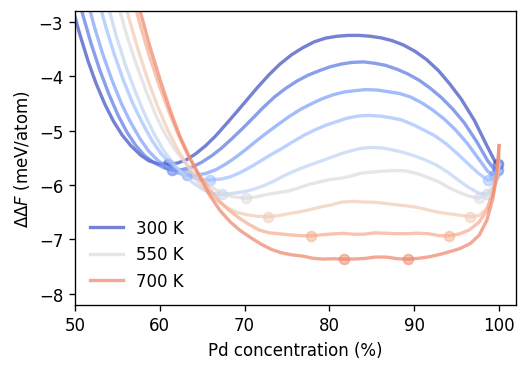
To demonstrate this approach we show below the relative mixing energy of mixing \(\Delta\Delta F\), which is obtained by removing the slope obtained via the convex hull/common tangent construction. The solubility limits/tangental points are indicated by the circles.

fig, ax = plt.subplots(
    figsize=(4.5, 3.2),
    dpi=120,
)

for temperature, df in results_vcsgc.groupby('temperature'):
    if temperature > 700:
        continue
    try:
        record = boundaries_vcsgc[boundaries_vcsgc.temperature == temperature].iloc[0]
    except:
        continue

    # free energy
    color = cmap((temperature - tmin) / (tmax - tmin))
    label = f'{temperature:.0f} K' if temperature in [tmin, int((tmin + tmax) / 2), 700, tmax] else ''
    ax.plot(1e2 * df.conc_mean, df.freen + record.slope * (1 - df.conc_mean),
            label=label, alpha=0.7, lw=2, color=color)

    # solubility limits
    data = np.array([
        (record.solubility_left,
         record.freen_left  + record.slope * (1 - record.solubility_left)),
        (record.solubility_right,
         record.freen_right  + record.slope * (1 - record.solubility_right)),
    ])
    ax.scatter(1e2 * data[:, 0], data[:, 1], alpha=0.5, color=color)

ax.set_xlabel(r'Pd concentration (%)')
ax.set_ylabel(r'$\Delta\Delta F$ (meV/atom)')
ax.set_xlim(50, 102)
ax.set_ylim(-8.2, -2.8)
ax.legend(frameon=False)

fig.tight_layout()

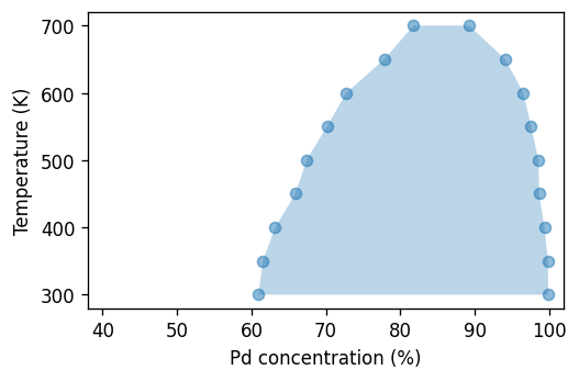
Finally, we can plot these data in the temperature-composition plane to obtain the phase diagram.

fig, ax = plt.subplots(
    figsize=(4.5, 3),
    dpi=120,
)

df = boundaries_vcsgc[boundaries_vcsgc.temperature < 720]

kwargs = dict(alpha=0.5, marker='o', color='C0')
ax.scatter(1e2 * df.solubility_left, df.temperature, **kwargs)
ax.scatter(1e2 * df.solubility_right, df.temperature, **kwargs)

ax.fill_betweenx(x1=1e2 * df.solubility_left, y=df.temperature,
                 x2=1e2 * df.solubility_right, alpha=0.3)

ax.set_xlabel(r'Pd concentration (%)')
ax.set_ylabel('Temperature (K)')
ax.set_xlim(38, 102)

fig.tight_layout()

SGC simulations

We now move on to the analysis of the SGC simulations and plot the variation of the composition with the chemical potential difference \(\Delta\mu\). Here, we focus on the \(\Delta\mu\) range close to the miscibility gap. We note, however, that in order to cover the full composition range \(\Delta\mu\) must be varied from around \(-0.6\) eV/atom to about \(+0.3\) eV/atom as can be seen in the figure comparing SGC and VCSGC above.

fig, ax = plt.subplots(
    figsize=(4.5, 3.2),
    dpi=120,
    sharex=True,
    sharey=True,
)

for temperature, df in results_sgc.groupby('temperature'):
    color = cmap((temperature - tmin) / (tmax - tmin))
    label = rf'{temperature:.0f} K'  if temperature in [tmin, tmax, int((tmin + tmax) / 2)] else ''
    for df2 in split_at_miscibility_gap(df, clim=0.15):
        ax.plot(1e2 * df2.conc_mean, df2.dmu, 'o-',
                label=label, alpha=0.8, lw=1, markersize=5, color=color)
        label = ''

ax.set_ylim(-0.58, 0.36)
ax.set_ylabel(r'$\partial F/\partial c$ and $\Delta\mu$ (eV/atom)')
ax.set_xlabel(r'Pd concentration (%)')

ax.set_xlim(50, 102)
ax.set_ylim(0.09, 0.33)
ax.legend(frameon=False, reverse=True)

fig.tight_layout()

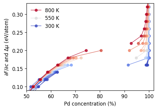
As described above the two-phase region shows up in this plot as a gap in the sampled composition range. While the variation of the boundaries with temperature is relatively smooth one can observe that some points appear to lie inside this range. This applies, e.g., for the data point at \(\Delta\mu=0.16\) eV/atom and 350 K. For this case as well as the two neighboring points the variation of the concentration with MC cycle is shown below.

fig, ax = plt.subplots(
    figsize=(4.5, 3.2),
    dpi=120,
    sharex=True,
    sharey=True,
)

for dmu in [0.140, 0.160, 0.180]:
    dc = DataContainer.read(f'runs-sgc/sgc-T350-dmu{dmu:.3f}-size6.dc')
    df = dc.data
    nsites = len(dc.structure)
    ax.plot(df.mctrial / nsites, 1e2 * df.Pd_count / nsites,
            alpha=0.6, label=f'{dmu:.3f} eV/atom')

ax.set_xlabel('MC cycle')
ax.set_ylabel(r'Pd concentration (%)')

fig.tight_layout()

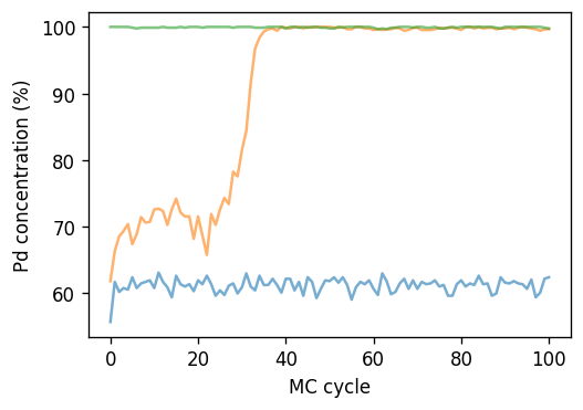
It is apparent that this simulation is not equilibrated until about 40 MC cycles, which is notably longer than the equilibration period that we considered during the compilation of the results.

We also note that the variation of \(\Delta\mu(c)\) close to the gap can be quite rapid and the spacing of data points along \(\Delta\mu\) is rather sparse. In this region a denser sampling is thus indicated.

When using the SGC ensemble one therefore commonly employs a boundary tracking approach that involves sampling closer and closer to the gap and finding the solubility limits through an iterative procedure as described in Model. Simul. Mater. Sci. Eng. 10, 521 (2002). We do not pursue this here further but note that the algorithm is straightforward to implement with little effort using the building blocks shown above.

Short-range order

Often it is insightful to also consider the variation of other observables as a function of temperature and/or composition. In part 3a of this tutorial we saw, e.g., that the heat capacity exhibits a characteristic variation with temperature across an order-disorder transition. Here, let us investigate the short-range order (SRO) in this system using the Warren-Cowley SRO parameter. The latter is even accessible via diffraction experiments and can therefore serve as a useful connection to experiment.

fig, ax = plt.subplots(
    figsize=(4.5, 3),
    dpi=120,
)

# short-range order parameter
sro = ax.tricontourf(1e2 * results_vcsgc.conc_mean,
                     results_vcsgc.temperature,
                     results_vcsgc.sro_Ag_1_mean,
                     cmap='RdBu_r', levels=40)
cbar = fig.colorbar(sro, ax=ax)
cs = np.linspace(-0.1, 0.1, 3)
cbar.set_ticks(ticks=cs, labels=cs)

# overlay phase boundaries from free energy analysis
df = boundaries_vcsgc[boundaries_vcsgc.temperature < 720]
conc = np.vstack([df.solubility_left, df.solubility_right]).flatten()
temp = np.vstack([df.temperature, df.temperature]).flatten()
df = DataFrame(np.array([conc, temp]).T, columns=['concentration', 'temperature'])
df.sort_values('concentration', inplace=True)
ax.plot(1e2 * df.concentration, df.temperature,
        'o-', color='0.5', alpha=0.8, markersize=5)

ax.set_xlabel(r'Pd concentration (%)')
ax.set_ylabel('Temperature (K)')

fig.subplots_adjust(hspace=0.2)

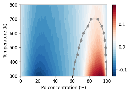
The figure reveals a pronounced dependence of the SRO parameter on composition and temperature. While the values are negative in the Ag-rich single-phase region of the phase diagram, one observes positive SRO parameters inside the miscibility gap. While the former is the result of the effective attractive interaction between Ag and Pd, the latter is the result of the coexistence of the Ag and Pd-rich phases. This behavior is analyzed in detail in Physical Review B 77, 134206 (2008) for the Fe-Cr system.

The figure also clearly shows that the SRO parameter is not a good predictor for the phase boundaries, at least not for these system sizes.

Tip: The SRO parameter assumes its minimal value around 25% Pd, which is in fact the result of an order-disorder transition at this composition. This is akin to the case of \(\ce{AuPd3}\) that was explored in part 3a of this tutorial series. You could adapt those scripts for the present system and explore this aspect in more detail.