Canonical ensemble

This tutorial demonstrates how to use Monte Carlo (MC) simulations to sample the canonical ensemble. The latter is well suited to sample order-disorder transitions at constant composition. To illustrate this aspect we consider the Au-Pd system, which exhibits a well-known order-disorder transition at 75% Pd. While the system is disordered at higher temperatures it assumes the so-called \(L1_2\) structure at low temperatures. For the simulations we use a cluster expansion for the AuPd:H system from the literature (Acta Materialia 211, 116893 (2021)), considering only the H-free system.

Running the simulations

Running MC simulations can take some time and commonly involves sampling over a range of temperatures or compositions. We therefore recommend to carry out these runs via regular python scripts (as opposed to running them in a notebook). The script for running the MC simulations for the present case can be found here.

In the following we provide a much abbreviated version that illustrates the working principle. For the analysis below, we will, however, resort to the “full” results generated by the script.

Load cluster expansion

We start by loading the cluster expansion (CE). One can show a short overview of the CE by printing the object. This can be achieved via print(ce). In jupyter notebooks one can also obtain an HTML formatted version via the display command, which is implied if the variable is stated on the last line of a cell (as done here).

from icet import ClusterExpansion

ce = ClusterExpansion.read('AuPd.ce')
ce

Cluster Expansion

Field	Value
Space group	Fm-3m (225)
Sublattice A	('Au', 'Pd')
Sublattice B	('H', 'X')
Cutoffs	[7. 5.]
Total number of parameters (nonzero)	63 (63)
Number of parameters of order 0 (nonzero)	1 (1)
Number of parameters of order 1 (nonzero)	2 (2)
Number of parameters of order 2 (nonzero)	18 (18)
Number of parameters of order 3 (nonzero)	42 (42)
fractional_position_tolerance	2e-06
position_tolerance	1e-05
symprec	1e-05

Prepare structure

Next we prepare the primitive structure. Here, we are using a cluster expansion that has been constructed to describe the AuPd:H system (doi:10.1016/j.actamat.2021.116893). We are, however, only interested in the H-free case. We therefore set the species on the H-lattice to “X”, which implies a vacancy.

primitive_structure = ce.primitive_structure
primitive_structure.symbols = ['Au', 'X']

We can now also set up supercell structure for the simulation. The primitive structure is based on an FCC lattice. To maximize the spacing between equivalent sites (and also for ease of visualization) it is preferable to use a conventional (simple cubic) cell. We therefore first convert the FCC lattice to the conventional cell.

import numpy as np
from ase.build import make_supercell

supercell = make_supercell(
    primitive_structure, [[-1, 1, 1], [1, -1, 1], [1, 1, -1]])

Then we repeat the cell and finally set the occupation of the Au/Pd lattice to the desired Pd concentration of 75%. Note that we can obtain an abbreviated view of the structure (an ase.Atoms object) by stating the variable on the last line of the cell, using the same implied display mechanism as above.

size = 4  # number of unit cells per direction
supercell = supercell.repeat(size)

concentration = 0.75  # Pd concentration
available_sites = [a.index for a in supercell if a.symbol == 'Au']
n_Pd = int(concentration * len(available_sites))
selection = np.random.choice(available_sites, size=n_Pd, replace=False)
supercell.symbols[selection] = 'Pd'
supercell

Atoms(symbols='Au64Pd192X256', pbc=True, cell=[16.0, 16.0, 16.0])

Set up a cluster expansion calculator

During a MC simulation one needs to evaluate the underlying cluster expansion many times. In order to do this in a computationally efficient manner, in icet one uses a calculator object that is specific for a particular supercell. Here, we therefore set up such a calculator.

As noted above, we are using a cluster expansion that has been constructed to describe the AuPd:H system. We are, however, only interested in the Au-Pd lattice. To sample the energy per Au/Pd atom (rather than per both Au/Pd and H/vacancy sites), we therefore overwrite the default scaling parameter, which is scaling=len(supercell), with scaling=len(supercell) / 2. In the vast majority of cases, such consideration is not needed but the present situation serves as a useful demonstration for the (occasional) utility of the scaling keyword.

from mchammer.calculators import ClusterExpansionCalculator

calculator = ClusterExpansionCalculator(supercell, ce, scaling=len(supercell) / 2)

Set up the ensemble object

The next step is to configure an ensemble object, which is then used to run the MC simulation. By default the interval at which data is saved equals the number of sites in the supercell, which is a sensible choice for production runs. Here, we shorten this interval in order to also demonstrate the equilibration period.

from mchammer.ensembles import CanonicalEnsemble

temperature = 170  # temperature in K at which to run the simulation
n_sites = int(len(supercell) / 2)  # number of sites on Au/Pd lattice
interval = int(n_sites / 16)
mc = CanonicalEnsemble(
    supercell,
    calculator=calculator,
    temperature=temperature,
    ensemble_data_write_interval=interval,
)

Attaching observers

In addition to say the energy, one is often interested in other observables such as, e.g., short or long-range order parameters, site occupancy factors. In icet this can be handled by attaching observer objects to the ensemble object. Here we are interested in the long-range order and the emergence of the \(L1_2\)-ordered structure, which can be observed by monitoring the static structure factor. The latter is given by

\[S(\mathbf{q}) \propto \sum_{j,k}^{N}e^{-i\mathbf{q}\cdot(\mathbf{R}_k - \mathbf{R}_j)}\]

and the \(\mathbf{q}\)-point of interest is \(\mathbf{q} = 2\pi/a_0 \left<100\right>\), where \(a_0\) is the lattice parameter.

from mchammer.observers import StructureFactorObserver

lattice_parameter = np.linalg.norm(supercell.cell, axis=1)[0]
qpoints = 2 * np.pi / lattice_parameter * np.eye(3)
LRO = StructureFactorObserver(
    supercell,
    q_points=qpoints,
    symbol_pairs=[['Pd', 'Pd'], ['Au', 'Au']],
    interval=interval,
)
mc.attach_observer(LRO)

Run the simulation

Finally we are ready to launch the simulation. Here, we run \(N_\mathrm{cycles}\) MC cycles, corresponding to \(N_\mathrm{cycles} \times N_\mathrm{sites}\) MC trials, where \(N_\mathrm{sites}\) is the number of Au and Pd sites. For the purpose of this demonstration we only run for a small number of MC cycles. In production larger value are recommended. Generally speaking the smaller the acceptance probability the more MC cycles are needed for convergence.

%%time
mc_cycles = 40
mc.run(n_sites * mc_cycles)

CPU times: user 9.68 s, sys: 384 ms, total: 10.1 s
Wall time: 9.57 s

Analyzing a simulation

The results of a MC simulation are available in the form of a data container object.

dc = mc.data_container
dc

Data Container

Field	Value
Type	DataContainer
n_atoms	512
n_atoms_Au	64
n_atoms_H	0
n_atoms_Pd	192
n_atoms_X	256
temperature	170
date_created	2024-04-29T08:08:41
ensemble_name	CanonicalEnsemble
hostname	pieweack
icet_version	2.2
seed	8139831348998210
user_tag	None
username	erhart
Number of rows in data	641

Using this object we can readily analyze various properties of interest. We can for example plot the energy as well as other observables as a function of MC trial step. These data are provided in the form of a DataFrame via the data property.

dc.data

	mctrial	potential	acceptance_ratio	sfo_Au_Au_q0	sfo_Au_Au_q1	sfo_Au_Au_q2	sfo_Pd_Pd_q0	sfo_Pd_Pd_q1	sfo_Pd_Pd_q2	total_q0	total_q1	total_q2
0	0	-10.101283	0.0000	0.082309	0.232479	0.081198	0.082309	0.232479	0.081198	0.164618	0.464959	0.162397
1	16	-10.405517	0.7500	0.073941	0.093750	0.086885	0.073941	0.093750	0.086885	0.147882	0.187500	0.173771
2	32	-10.510665	0.1875	0.166906	0.041188	0.080413	0.166906	0.041188	0.080413	0.333812	0.082376	0.160826
3	48	-10.560768	0.4375	0.138729	0.113396	0.117188	0.138729	0.113396	0.117188	0.277459	0.226792	0.234375
4	64	-10.779601	0.5000	0.020594	0.260656	0.343520	0.020594	0.260656	0.343520	0.041188	0.521312	0.687040
...	...	...	...	...	...	...	...	...	...	...	...	...
636	10176	-11.739776	0.1250	0.131539	0.001340	0.031643	0.131539	0.001340	0.031643	0.263079	0.002681	0.063285
637	10192	-11.689833	0.1250	0.221106	0.002288	0.067469	0.221106	0.002288	0.067469	0.442211	0.004576	0.134938
638	10208	-11.696855	0.2500	0.244706	0.062500	0.001178	0.244706	0.062500	0.001178	0.489411	0.125000	0.002356
639	10224	-11.677870	0.1250	0.166581	0.086885	0.015855	0.166581	0.086885	0.015855	0.333161	0.173771	0.031710
640	10240	-11.698306	0.2500	0.162397	0.120424	0.050341	0.162397	0.120424	0.050341	0.324794	0.240847	0.100682

641 rows × 12 columns

from matplotlib import pyplot as plt

fig, axes = plt.subplots(
    figsize=(4.5, 4.2),
    dpi=120,
    nrows=2,
    sharex=True,
)

ax = axes[0]
ax.plot(dc.data.mctrial / n_sites, 1e3 * dc.data.potential / n_sites)
ax.set_ylabel('$E_\mathrm{mix}$ (meV/atom)')

ax = axes[1]
ax.plot(dc.data.mctrial / n_sites, 1e2 * dc.data.acceptance_ratio)
ax.set_ylabel(r'Acceptance ratio (%)')
ax.set_xlabel('MC cycle')

fig.align_ylabels()
fig.subplots_adjust(hspace=0)

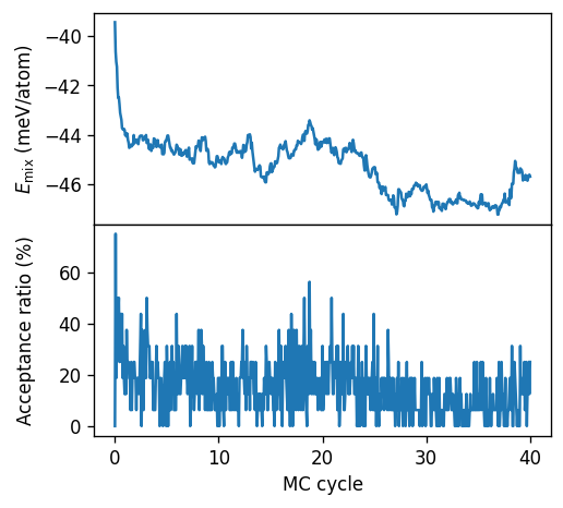
From the figure above we can observe that for this system at this temperature requires at least 20 to 30 MC cycles to reach an equilibrated state.

Finally we note that one can access the trajectory in the form of a list of ase.Atoms objects via dc.get('trajectory').

Compiling the results

We will now analyze the results of the MC simulations that have been carried out using the script. For convenience (and to avoid unnecessary repetition) the results of the MC simulations are available for download via zenodo. When working on the command line one can download them for example by running the following command.

wget https://zenodo.org/records/10997198/files/runs-canonical.zip
unzip runs-canonical.zip

Afterwards the results should be available in the form of *.dc files in the runs-canonical directory. We can then loop over these files and compute thermodynamic averages along with error estimates. In the following we use the analyze_data() method of the DataContainer object to compute the mean, standard deviation, correlation time, and error estimate (95% confidence interval) for the potential sampled in the MC simulation (i.e., the mixing energy) as well as the structure factor. From the standard deviation of the energy \(\sigma_E\) we can then compute the heat capacity via

\[C_V = \frac{\sigma_E^2}{k_BT^2}.\]

Furthermore we compute the average of the structure factor over the three Cartesian directions.

Note that the following cell takes several minutes to evaluated when using the data provided for this tutorial.

%%time

from glob import glob
from ase.units import kB
from mchammer import DataContainer
from pandas import DataFrame

# suppress RuntimeWarnings due to division by zero
np.seterr(invalid='ignore')

data = []
for fname in sorted(glob('runs-canonical/*.dc')):
    dc = DataContainer.read(fname)
    n_sites = int(len(dc.structure) / 2)
    record = dict(
        temperature=dc.ensemble_parameters['temperature'],
        n_sites=n_sites,
        n_samples=len(dc.data),
    )
    data.append(record)
    for prop in ['potential',
                 'sfo_Pd_Pd_q0', 'sfo_Pd_Pd_q1', 'sfo_Pd_Pd_q2',
                 'acceptance_ratio']:
        # drop the first 100 MC cycles for equilibration
        result = dc.analyze_data(prop, start=100 * n_sites)
        record.update({f'{prop}_{key}': value for key, value in result.items()})

# convert list of dicts to DataFrame
results = DataFrame.from_dict(data)

# add heat_capacity and average structure factor (sfo)
results['heat_capacity'] = results.potential_std ** 2 / kB / results.temperature ** 2
results['heat_capacity'] /= kB * results.n_sites
results['sfo'] = (results.sfo_Pd_Pd_q0_mean +
                  results.sfo_Pd_Pd_q1_mean +
                  results.sfo_Pd_Pd_q2_mean) / 3 / results.n_sites

CPU times: user 4min 9s, sys: 398 ms, total: 4min 9s
Wall time: 4min 10s

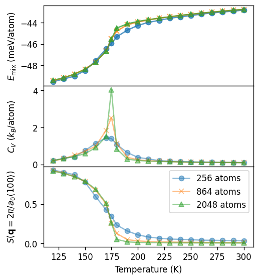
Analyzing the results

Finally we can plot the thermodynamic averages. The order-disorder transition is apparent in both the heat capacity and the structure factor. In particular in the case of the heat capacity one finds a clear peak at about 175 K, illustrating the continuous character of this transition. One can also observe a pronounced size dependence, which is characteristic for this transition type.

fig, axes = plt.subplots(
    figsize=(4.5, 5.2),
    dpi=120,
    nrows=3,
    sharex=True,
)

for k, (n_sites, df) in enumerate(results.groupby('n_sites')):
    kwargs = dict(
        label=f'{n_sites} atoms',
        color=f'C{k}',
        marker='ox^v'[k],
        alpha=0.5,
    )
    axes[0].plot(df.temperature, 1e3 * df.potential_mean / n_sites, **kwargs)
    axes[0].errorbar(df.temperature, 1e3 * df.potential_mean / df.n_sites,
                     yerr=1e3 * df.potential_error_estimate / df.n_sites, **kwargs)
    axes[1].plot(df.temperature, df.heat_capacity, **kwargs)
    axes[2].plot(df.temperature, df.sfo / 0.065, **kwargs)

axes[0].set_ylabel('$E_\mathrm{mix}$ (meV/atom)')
axes[1].set_ylabel('$C_V$ ($k_B$/atom)')
axes[2].set_ylabel(r'$S(\mathbf{q}=2\pi/a_0\left<100\right>)$')
axes[-1].set_xlabel('Temperature (K)')
axes[-1].legend()

fig.align_ylabels()
fig.subplots_adjust(hspace=0)

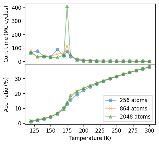
It is instructive to analyze the convergence of the simulations at different temperatures. The figure below shows both the correlation time of the potential and the acceptance ratio. Since the acceptance ratio drops with temperature, longer runs (more trials) are required to converge averages at lower temperatures. It is also apparent that the temperature dependence of the acceptance ratio mimics that of the potential, suggesting that the presence of the transition itself increases the need for sampling.

The latter aspect is even more apparent from the correlation time, which exhibits divergent behavior around the transition, reflecting the divergence of the fluctuations (such as the heat capacity) at the transition. Converging the thermodynamic averages in the vicinity of the transition therefore demands very extensive sampling, a requirement that becomes even more dramatic with increasing system size.

fig, axes = plt.subplots(
    figsize=(4.5, 4.2),
    dpi=120,
    nrows=2,
    sharex=True,
)

for k, (n_sites, df) in enumerate(results.groupby('n_sites')):
    kwargs = dict(
        label=f'{n_sites} atoms',
        color=f'C{k}',
        marker='ox^v'[k],
        alpha=0.5,
    )
    axes[0].plot(df.temperature, df.potential_correlation_length / df.n_sites, **kwargs)
    axes[1].plot(df.temperature, 1e2 * df.acceptance_ratio_mean, **kwargs)

axes[0].set_ylabel(r'Corr. time (MC cycles)')
axes[1].set_ylabel(r'Acc. ratio (%)')
axes[-1].set_xlabel('Temperature (K)')
axes[-1].legend()

fig.align_ylabels()
fig.subplots_adjust(hspace=0)

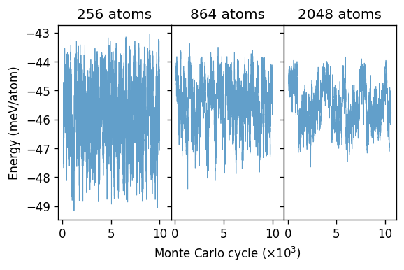
To demonstrate the correlation time it is instructive to plot the potential (i.e., here the mixing energy) as a function of MC cycle. Here, we specifically consider the systems at the critical temperature of 175 K, for which the correlation times are the longest.

In particular the largest system one can clearly see how the system appears to move between two different energy regions, which should approximately correspond to ordered (lower energy) and disordered (higher energy) structures. For the 864-atoms system this effect is still somewhat visible but for the 256-atoms system it is washed out as the transition between the two structure types happens readily and very frequently.

From these plots it is also apparent why such long runs are required to achieve convergence in the vicinity of the critical temperature, as one must sample multiple times longer than the correlation time.

fig, axes = plt.subplots(
    figsize=(5.2, 3),
    dpi=120,
    ncols=3,
    sharex=True,
    sharey=True,
)

for icol, size in enumerate([4, 6, 8]):
    dc = DataContainer.read(f'runs-canonical/T175-size{size}.dc')
    n_sites = int(len(dc.structure) / 2)
    df = dc.data
    df = df[df.mctrial / n_sites > 100]

    ax = axes[icol]
    ax.plot(1e-3 * df.mctrial / n_sites, 1e3 * df.potential / n_sites, alpha=0.7, lw=0.5)
    ax.set_title(f'{n_sites} atoms')

axes[0].set_ylabel('Energy (meV/atom)')
axes[1].set_xlabel(r'Monte Carlo cycle ($\times 10^3$)')

fig.subplots_adjust(wspace=0)

The appearance of both ordered and disordered motifs in a single trajectory is characteristic of a critical system. As we have seen in the previous figure, the different motifs are associated with slightly different energies. At temperatures above or below the transition only one structural motif occurs with high probability. This is illustrated by the energy histograms below.

from matplotlib import colormaps

fig, axes = plt.subplots(
    figsize=(5.2, 3),
    dpi=120,
    ncols=3,
    sharex=True,
    sharey=True,
)

temperatures = [160, 170, 175, 180, 190]
tmin, tmax = np.min(temperatures), np.max(temperatures)
cmap = colormaps['coolwarm']

for icol, size in enumerate([4, 6, 8]):
    ax = axes[icol]
    for temperature in temperatures:

        # load data
        dc = DataContainer.read(f'runs-canonical/T{temperature}-size{size}.dc')

        # remove equilibration period
        n_sites = int(len(dc.structure) / 2)
        df = dc.data
        df = df[df.mctrial / n_sites > 100]

        # compute histogram
        hist, bins = np.histogram(
            1e3 * df.potential / n_sites,
            range=(-51, -42), density=True, bins=200)
        # The histogram function returns bin _boundaries_ but below
        # we plot the histogram using the _centers_ of the bins.
        # Here we therefore shift the bins by half a bin width.
        bins = bins[:-1] + (bins[1] - bins[0]) / 2

        color = cmap((temperature - tmin) / (tmax - tmin))
        ax.plot(bins, hist, label=f'{temperature} K', color=color)
    ax.set_title(f'{n_sites} atoms')

axes[0].set_ylabel('Relative occurence')
axes[1].set_xlabel('Energy (meV/atom)')
axes[0].legend()

fig.subplots_adjust(wspace=0)

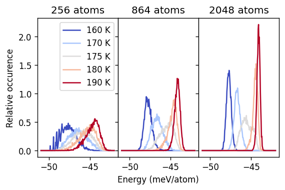
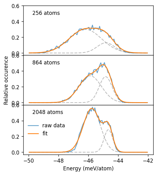
For temperatures above or below the transition the distribution is sharp. By contrast at 175 K and thus near the critical temperature, the distribution is much broader. In particular for the largest system size considered here, one can anticipate the emergence of a bimodal distribution at 175 K, with the two modes corresponding to the two distinct structural motifs sampled.

To bring out the latter point below we decompose the energy at 175 K into two normal distributions, corresponding, respectively to the ordered and disordered motifs.

from scipy.optimize import curve_fit

def normal_distribution(x, mu, sig):
    return 1 / sig / np.sqrt(2 * np.pi) * np.exp(-0.5 * ((x - mu) / sig) ** 2)

def func(x, mu1, sig1, mu2, sig2, A1, A2):
    f = A1 * normal_distribution(x, mu1, sig1)
    f += A2 * normal_distribution(x, mu2, sig2)
    return f


fig, axes = plt.subplots(
    figsize=(4.5, 5.2),
    dpi=120,
    nrows=3,
    sharex=True,
    sharey=True,
)

for irow, size in enumerate([4, 6, 8]):

    # load data
    dc = DataContainer.read(f'runs-canonical/T175-size{size}.dc')

    # remove equilibration period
    n_sites = int(len(dc.structure) / 2)
    df = dc.data
    df = df[df.mctrial / n_sites > 100]

    # compute histogram
    hist, bins = np.histogram(
        1e3 * df.potential / n_sites,
        range=(-50, -42), density=True, bins=100)
    bins = bins[:-1] + (bins[1] - bins[0]) / 2

    # fit histogram to double Gaussian
    p0 = (-47, 1, -44, 1, 1, 1)
    pars, _ = curve_fit(func, bins, hist, p0=p0)
    mu1, sig1, mu2, sig2, A1, A2 = pars

    ax = axes[irow]
    ax.text(0.07, 0.82, f'{n_sites} atoms', transform=ax.transAxes)

    kwargs = dict(color='0.5', alpha=0.5, ls='--')
    ax.plot(bins, A1 * normal_distribution(bins, mu1, sig1), **kwargs)
    ax.plot(bins, A2 * normal_distribution(bins, mu2, sig2), **kwargs)

    ax.plot(bins, hist, alpha=0.7, label='raw data')
    ax.plot(bins, func(bins, mu1, sig1, mu2, sig2, A1, A2), label='fit')

axes[1].set_ylabel('Relative occurence')
axes[-1].set_xlabel('Energy (meV/atom)')
axes[-1].legend(loc='center left', frameon=False)

fig.subplots_adjust(hspace=0)