Additional material
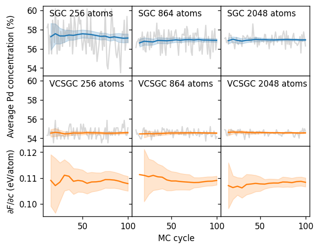
Convergence of simulations
[784]:
from mchammer.data_analysis import analyze_data

fig, axes = plt.subplots(
    figsize=(5.8, 4.6),
    dpi=120,
    nrows=3,
    ncols=3,
    sharex=True,
    sharey='row',
)

temperature = 300
dmu, phi = 0.140, -1.250
dmu, phi = 0.120, -1.175
#dmu, phi = 0.000, -0.775
kappa = 50

# Number of MC cyclces to remove from the beginning of
# the trajectory to account for equilibration.
mcc_cutoff = 10

for icol, size in enumerate([4, 6, 8]):
    for irow, ensemble in enumerate(['sgc', 'vcsgc']):

        # load data container
        if ensemble == 'sgc':
            fname = f'runs/sgc-T{temperature}-dmu{dmu:.3f}-size{size}.dc'
        else:
            fname = f'runs/vcsgc-T{temperature}-phi{phi:.3f}-kappa{kappa}-size{size}.dc'
        dc = DataContainer.read(fname)

        # add columns with MC cycle and concentration
        df = dc.data
        n_sites = len(dc.structure)
        df['mccycle'] = df.mctrial / n_sites
        df['conc'] = df.Pd_count / n_sites

        # remove equilibration period
        df = df[df.mccycle > mcc_cutoff]

        # compute averages for trajectories of different length (nmax)
        data = []
        for nmax in range(mcc_cutoff + 5, 100 + 1, 5):
            record = dict(nmax=nmax)
            data.append(record)
            res = analyze_data(df[df.mccycle <= nmax].conc)
            record.update({f'conc_{k}': v for k, v in res.items()})
            if ensemble == 'vcsgc':
                res = analyze_data(df[df.mccycle <= nmax].free_energy_derivative_Pd)
                record.update({f'dfreen_{k}': v for k, v in res.items()})
        df_avg = DataFrame.from_dict(data)

        # plot mean concentration and error estimate
        ax = axes[irow][icol]
        color = 'C0' if ensemble == 'sgc' else 'C1'
        ax.text(0.07, 0.85, f'{ensemble.upper()} {n_sites} atoms', transform=ax.transAxes)
        ax.plot(df.mccycle, 1e2 * df.conc, color='0.5', alpha=0.3)
        ax.plot(df_avg.nmax, 1e2 * df_avg.conc_mean, color=color)
        ax.fill_between(df_avg.nmax,
                        y1=1e2 * (df_avg.conc_mean - df_avg.conc_error_estimate),
                        y2=1e2 * (df_avg.conc_mean + df_avg.conc_error_estimate),
                        color=color, alpha=0.2)

        # plot mean free energy derivative and error estimate (VCGSC only)
        if ensemble == 'vcsgc':
            color = 'C1'
            ax = axes[2][icol]
            ax.plot(df_avg.nmax, df_avg.dfreen_mean, color=color)
            ax.fill_between(df_avg.nmax,
                        y1=df_avg.dfreen_mean - df_avg.dfreen_error_estimate,
                        y2=df_avg.dfreen_mean + df_avg.dfreen_error_estimate,
                        color=color, alpha=0.2)

axes[1][0].set_ylim(axes[0][0].get_ylim())

axes[1][0].set_ylabel(r'Average Pd concentration (%)', y=1)
axes[2][0].set_ylabel(r'$\partial F/\partial c$ (eV/atom)')
axes[-1][1].set_xlabel(r'MC cycle')

fig.subplots_adjust(wspace=0, hspace=0)
fig.align_ylabels()
The VCSCG variance constraint \(\bar{\kappa}\)
The VCSGC ensemble requires one to specify both an average and a variance constraint for the concentration. So far we have used the recommended default value of \(\bar{\kappa}=200\). It is now instructive to explore this aspect in a bit more detail. To this end, we first repeat the previous VCSGC-MC simulations for several different values of \(\bar{\kappa}\).
[15]:
%%time

for kappa in [5, 10, 50, 500]:
    for phi in phis:
        mc = VCSGCEnsemble(
            supercell,
            calculator=calculator,
            temperature=temperature,
            phis={'Pd': phi},
            kappa=kappa,
        )
        mc.run(len(supercell) * mc_cycles)
        dcs_vcsgc[(phi, kappa)] = mc.data_container
CPU times: user 1min 22s, sys: 264 ms, total: 1min 22s
Wall time: 1min 23s
We compile the results in a DataFrame for convenient analysis.
[16]:
data = []
for (phi, kappa), dc in dcs_vcsgc.items():
    n_sites = len(dc.structure)
    Pd_count = dc.analyze_data('Pd_count', start=mcc_cutoff * n_sites)
    accratio = dc.analyze_data('acceptance_ratio', start=mcc_cutoff * n_sites)
    dfreen = dc.analyze_data(
            'free_energy_derivative_Pd', start=mcc_cutoff * n_sites)
    data.append(dict(
        phi=phi,
        kappa=kappa,
        Pd_conc=Pd_count['mean'] / n_sites,
        Pd_conc_err=Pd_count['error_estimate'] / n_sites,
        Pd_conc_std=Pd_count['std'] / n_sites,
        Pd_conc_corr=Pd_count['correlation_length'],
        acceptance_ratio=accratio['mean'],
        free_energy_derivative=dfreen['mean'],
        free_energy_derivative_err=dfreen['error_estimate'],
    ))
df_vcsgc = DataFrame.from_dict(data)
[741]:
%%time

from glob import glob

files = sorted(glob('runs/vcsgc-T300-phi*-kappa2-size6.dc'))
df_vcsgc = collect_data(files)
100%|██████████| 248/248 [00:18<00:00, 13.09it/s]
CPU times: user 18.7 s, sys: 80.6 ms, total: 18.8 s
Wall time: 19 s
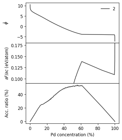
Below we plot the results, which allows us to make several relevant observations.
In VCSGC-MC simulations one obtains a nearly linear mapping between the average constraint parameter \(\bar{\phi}\) and the average concentration \(\left<c\right>\). This is consistent with the observation made above that the VCSGC-MC simulations yielded a more even sampling of the concentration range than the SGC-MC simulations.
When increasing \(\bar{\kappa}\), the concentration range sampled for a fixed range of \(\bar{\phi}\) increases. When \(\bar{\kappa}\) approaches zero on the other hand, the VCSGC ensemble maps back to the SGC ensemble.
The free energy derivative is independent of the choice of \(\bar{\kappa}\).
The acceptance ratio drops, however, with increasing \(\bar{\kappa}\), which means that longer runs are needed to achieve convergence.
[755]:
fig, axes = plt.subplots(
    figsize=(4, 5.2),
    dpi=120,
    nrows=3,
    sharex=True,
)

log_kappa_min = np.log(df_vcsgc.kappa.min())
log_kappa_max = np.log(df_vcsgc.kappa.max())

for kappa, df in df_vcsgc.groupby('kappa'):
    if kappa < 5:
        continue
    kwargs = dict(
        alpha=0.7,
        label=f'{kappa}' if kappa in [2, 50, 500] else '',
        color=cmap((np.log(kappa) - log_kappa_min) / (log_kappa_max - log_kappa_min)),
    )
    axes[0].plot(1e2 * df.conc_mean, df.phi, **kwargs)
    axes[1].plot(1e2 * df.conc_mean, df.free_energy_derivative_Pd_mean, **kwargs)
    axes[2].plot(1e2 * df.conc_mean, 1e2 * df.acceptance_ratio_mean, **kwargs)

axes[-1].set_xlabel(r'Pd concentration (%)')
axes[0].set_ylabel(r'$\bar{\phi}$')
axes[1].set_ylabel(r'$\partial F/\partial c$ (eV/atom)')
axes[2].set_ylabel(r'Acc. ratio (%)')
axes[0].legend(ncol=3, frameon=False)

axes[1].set_ylim(0.09, 0.18)

fig.align_ylabels()
fig.subplots_adjust(hspace=0)
[722]:
fig, axes = plt.subplots(
figsize=(4, 5.2),
dpi=120,
nrows=3,
sharex=True,
)
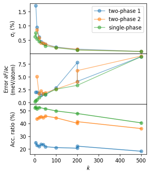
for k, (label, target_conc, tol) in enumerate([
('two-phase 1', 0.865, 0.01),
('two-phase 2', 0.726, 0.015),
('single-phase', 0.597, 0.004),
]):
df = df_vcsgc[np.isclose(df_vcsgc.conc_mean, target_conc, atol=tol)].sort_values('kappa')
df = df[df.kappa <= 500]
kwargs = dict(
color=f'C{k}',
alpha=0.5,
label=label,
)
ax = axes[0]
ax.plot(df.kappa, 1e2 * df.conc_std, 'o-', **kwargs)
ax.set_ylabel(r'$\sigma_c$ (%)')
ax = axes[1]
ax.plot(df.kappa, 1e3 * df.free_energy_derivative_Pd_error_estimate, 'o-', **kwargs)
ax.set_ylabel(r'Error $\partial F/\partial c$' + '\n(meV/atom)')
ax = axes[2]
"""
if '2' in label:
ax.plot(df.kappa, 1e2 * df.conc_mean, 'o-', **kwargs)
"""
ax.plot(df.kappa, 1e2 * df.acceptance_ratio_mean, 'o-', **kwargs)
ax.errorbar(df.kappa, 1e2 * df.acceptance_ratio_mean,
yerr=1e2 * df.acceptance_ratio_error_estimate, **kwargs)
ax.set_ylabel(r'Acc. ratio (%)')
axes[0].legend()
axes[-1].set_xlabel(r'$\bar{\kappa}$')
fig.align_ylabels()
fig.subplots_adjust(hspace=0)
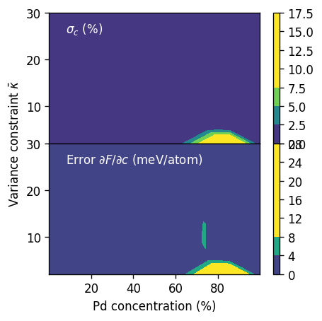
[723]:
fig, axes = plt.subplots(
    figsize=(4, 4),
    dpi=120,
    nrows=2,
    sharex=True,
    sharey=True,
)

df = df_vcsgc.dropna(subset='free_energy_derivative_Pd_error_estimate')
df = df[df.kappa <= 30]
#df = df[(df.conc_mean >= 0.6) & (df.conc_mean <= 0.9)]

ax = axes[0]
cm = ax.tricontourf(1e2 * df.conc_mean, df.kappa, 1e2 * df.conc_std, vmax=8)
plt.colorbar(cm, ax=ax)
pos = (0.08, 0.85)
ax.text(*pos, r'$\sigma_c$ (%)', transform=ax.transAxes, color='white')

ax = axes[1]
cm = ax.tricontourf(1e2 * df.conc_mean, df.kappa,
                    1e3 * df.free_energy_derivative_Pd_error_estimate, vmax=10)
plt.colorbar(cm, ax=ax)
ax.text(*pos, r'Error $\partial F/\partial c$ (meV/atom)', transform=ax.transAxes, color='white')

axes[-1].set_xlabel(r'Pd concentration (%)')
axes[1].set_ylabel(r'Variance constraint $\bar{\kappa}$', y=1)

fig.align_ylabels()
fig.subplots_adjust(hspace=0)
[ ]:
[ ]:
[ ]:
[ ]:
[ ]:
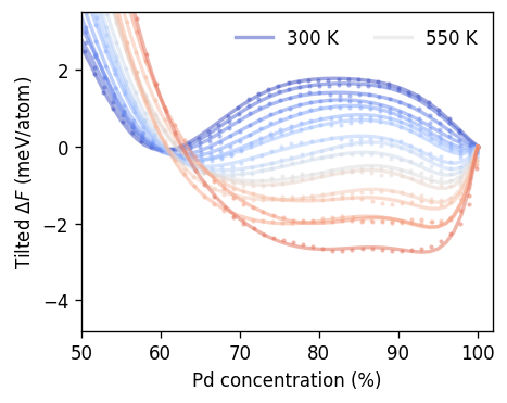
[406]:
from scipy.optimize import curve_fit

def rk_func(x, *pars):
    xmod = (x - pars[0]) / (1 - pars[0])
    f = 0
    for k, p in enumerate(pars[1:]):
        f += p * (1 - 2 * xmod) ** k * xmod  * (1 - xmod)
    return f


fig, ax = plt.subplots(
    figsize=(4, 3.2),
    dpi=120,
)

rk_order = 6

parameters = {}
for temperature, df in df_selection.groupby('temperature'):
    try:
        slope = boundaries_direct[boundaries_direct.temperature == temperature].iloc[0].slope
    except:
        continue

    df.dropna(subset='freen', inplace=True)
    df['freen_tilted'] = df.freen + slope * (1 - df.conc_mean)
    df = df[df.conc_mean > 0.5]
    pars, _ = curve_fit(rk_func, df.conc_mean, df.freen_tilted, p0=[0.6] + rk_order * [1])
    parameters[temperature] = pars

    color = cmap((temperature - tmin) / (tmax - tmin))
    ax.scatter(1e2 * df.conc_mean, df.freen_tilted, alpha=0.5, s=6, lw=0, color=color)

    xs = np.linspace(0, 1, 101)
    ax.plot(1e2 * xs, rk_func(xs, *pars),
            label=f'{temperature:.0f} K' if temperature in [tmin, 550, 750, tmax] else '',
            alpha=0.5, lw=2, color=color)

ax.set_xlabel(r'Pd concentration (%)')
ax.set_ylabel(r'Tilted $\Delta F$ (meV/atom)')
ax.set_xlim(50, 102)
ax.set_ylim(-4.8, 3.5)
ax.legend(frameon=False, ncol=3)

fig.tight_layout()
[407]:
from icet.tools import ConvexHull

xs = np.linspace(0.5, 1, 101)

data = []
for temperature, pars in parameters.items():
    ys = rk_func(xs, *pars)

    ch = ConvexHull(xs, ys)
    df_hull = DataFrame(np.array([ch.concentrations, ch.energies]).T,
                        columns=['conc_mean', 'freen'])
    dfs = split_at_miscibility_gap(df_hull, clim=0.04)
    if len(dfs) < 2:
        continue

    freen_left = dfs[-2].iloc[-1].freen
    freen_right = dfs[-1].iloc[0].freen
    conc_left = dfs[-2].iloc[-1].conc_mean
    conc_right = dfs[-1].iloc[0].conc_mean
    slope = (freen_right - freen_left) / (conc_right - conc_left)

    data.append(dict(
        temperature=temperature,
        conc_left=conc_left,
        conc_right=conc_right,
        slope=slope,
    ))

boundaries_interpolated = DataFrame.from_dict(data)
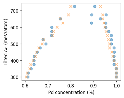
[410]:
fig, ax = plt.subplots(
    figsize=(4, 3.2),
    dpi=120,
)

kwargs = dict(alpha=0.5, marker='o', color='C0')
ax.scatter(boundaries_direct.conc_left,
           boundaries_direct.temperature, **kwargs)
ax.scatter(boundaries_direct.conc_right,
           boundaries_direct.temperature, **kwargs)

kwargs = dict(alpha=0.5, marker='x', color='C1')
ax.scatter(boundaries_interpolated.conc_left,
           boundaries_interpolated.temperature, **kwargs)
ax.scatter(boundaries_interpolated.conc_right,
           boundaries_interpolated.temperature, **kwargs)

ax.set_xlabel(r'Pd concentration (%)')
ax.set_ylabel(r'Tilted $\Delta F$ (meV/atom)')
#ax.set_xlim(50, 102)
#ax.set_ylim(-4.8, 3.5)
ax.legend(frameon=False, ncol=3)

fig.tight_layout()
No artists with labels found to put in legend. Note that artists whose label start with an underscore are ignored when legend() is called with no argument.