CE constructuon for low-symmetry systems

In this notebook, we construct cluster expansions (CE) for a low-symmetry system, namely a 12-layer AuPd FCC-(111) surface slab. Low symmetry systems are associated with a large number of inequivalent sites which results in a large number of parameters which can lead to issues.

In this tutorial, we will construct CEs using 4 different approaches:

1. Regular CE

2. CE with merged orbits

3. Bayesian CE

4. CE with weighted constraints

The training data (AuPd-111.db) consists of DFT mixing energies of 203 structures that have been relaxed and remapped to an ideal lattice as well as the 12 structures necessary for segregation energy calculations.

Regular CE

First, we construct a CE using the regular approach (similar to part 1 of this tutorial).

Set up a cluster space

We start by setting up a cluster space for our system. With [6.0, 3.0] as cutoffs, we get 76 parameters.

from ase.db import connect
from icet import ClusterSpace

# Database with training structures
db = connect('AuPd-111.db')

# Get primitive structure from pure Au
primitive = db.get(formula='Au12').toatoms()

# Set up cluster space
cs = ClusterSpace(structure=primitive,
                  cutoffs=[6.0, 3.0],
                  chemical_symbols=['Au', 'Pd'])
cs

Cluster Space

Field	Value
Space group	P-3m1 (164)
Sublattice A	('Au', 'Pd')
Cutoffs	[6.0, 3.0]
Total number of parameters	76
Number of parameters of order 0	1
Number of parameters of order 1	6
Number of parameters of order 2	46
Number of parameters of order 3	23
fractional_position_tolerance	1e-06
position_tolerance	1e-05
symprec	1e-05

Load training data

Then, we set up a structure container and add the structures that constitute the training data.

from icet import StructureContainer

# Set up structure container and add structures
sc = StructureContainer(cluster_space=cs)

for row in db.select():
    # For now, we skip the structures used for calculating the segregation energy
    if row.tag == 'se':
        continue

    structure = row.toatoms()

    # Add to structure container
    sc.add_structure(structure=structure,
                     properties={'mixing_energy': row.mixing_energy})

print(f'Number of structures: {len(sc)}')

Number of structures: 203

Train cluster expansion

Lastly, we train the model using cross validation and set up the cluster expansion.

The multiplicities can be included in either the sensing matrix or the ECI vector during training. The default behavoir in icet is to include them in the ECI vector, but in this notebook we will explicitly move them to the sensing matrix during training since that is necessary for the Bayesian approach we will use later on.

import numpy as np
from trainstation import CrossValidationEstimator
from icet import ClusterExpansion

# Get data for training
A, y = sc.get_fit_data(key='mixing_energy')

# Get the multiplicities
M = np.array(cs.get_multiplicities())

# Multiply the multiplicities with each column of the sensing matrix A
A = A*(M.T)

# Train using ARDR with `threshold_lambda=1e5`
fit_kwargs = dict(threshold_lambda = 1e5)
opt = CrossValidationEstimator(fit_data=(A,y), fit_method='ardr', **fit_kwargs)

# First do cross validation to get validation errors
opt.validate()
# Then train final model on the entire data set
opt.train()
print(opt)

# Extract ECIs
parameters = opt.parameters.copy()

# Multiply with multiplicities to obtain CEs in the standard `ICET` format
parameters *= M

# Generate cluster expansion
ce_regular = ClusterExpansion(cluster_space=cs, parameters=parameters)

============== CrossValidationEstimator ==============
seed                           : 42
fit_method                     : ardr
standardize                    : True
n_target_values                : 203
n_parameters                   : 76
n_nonzero_parameters           : 71
parameters_norm                : 0.06631216
target_values_std              : 0.02193294
rmse_train                     : 0.002033297
R2_train                       : 0.9909873
AIC                            : -2364.777
BIC                            : -2129.539
validation_method              : k-fold
n_splits                       : 10
rmse_train_final               : 0.002082207
rmse_validation                : 0.003519105
R2_validation                  : 0.9710606
threshold_lambda               : 100000
shuffle                        : True
======================================================

The final cluster expansion has 71 non-zero parameters and a validation error of 3.5 eV/atom.

Merged CE

Now will construct a CE with merged orbits. The merging is based on the idea that orbits (with a certain radius and order) in the bulk region should be similar, even if they are not symetrically equivallent due to the different surface layers and can therefore be represented by the same ECI. This is achieved by merging these orbit which reduces the number of parameters.

Inspecting orbits

In order to define the rules for merging, we need to be able to inspect the orbits. This can be done by iterating over the orbit list and obtaining certain properties of the orbit, such as the order, radius, involved sites and positions of the involved sites.

Below we exemplify using the 10th orbit. If we print the orbit, we get the order, multiplicity and radius as well as the sites and their respective unit cell offset for the representative cluster and all clusters in the orbit. We can also obtain the properties of interest as properties of the orbit object.

orb_index = 10
orb = cs.orbit_list[orb_index]

# Print an overview of the orbit
print(f'Overview of orbit {orb_index}:\n', orb)

# Print specific properties (of the representative cluster)
print(f'Specific properties of orbit {orb_index}:')
print(f'Order: {orb.order}, Sites: {orb.sites}, Radius: {orb.radius}')
print(f'Positions: {orb.positions}')

Overview of orbit 10:
 Order: 2
Multiplicity: 6
Radius: 1.4142
Representative cluster:
        Site: 1,        Offset:  -1 -1  0,      Position:  -1.41  -0.82  12.31
        Site: 2,        Offset:   0  0  0,      Position:   0.00   0.00  14.62

Specific properties of orbit 10:
Order: 2, Sites: [1, 2], Radius: 1.4142135623815457
Positions: [array([-1.41421356, -0.81649658, 12.30940108]), array([ 0.        ,  0.        , 14.61880215])]

Rules for merging

The merging is based on the following principle. The surface slab consists of 12 sites corresponding to the atomic layers. We consider the surface layer, i.e. sites 0 and 11, to be the surface and the remaining sites to be the bulk. All orbits with the same order and radius consisting of bulk sites only should be merged.

The information about which orbits to merge are provided as a dict where the key is an orbit index, and the corresponding value is a list of orbit indicies that should be merged with the key one. One could define the rules for merging manually by inspecting the relevant properties as shown above. This becomes tedious for larger systems, so instead we write an algorithm to do it automatically by comparing the order, radius and and sites of all orbits.

# Define surface vs. bulk sites
surface_sites = [0, 11]
bulk_sites = [1, 2, 3, 4, 5, 6, 7, 8, 9, 10]

# Dictonary to keep track of orbits to merge
merge_info = {}

# Loop over all orbits
for i, orb in enumerate(cs.orbit_list):
    # Check if all sites are bulk (if yes - merge)
    if all(site in bulk_sites for site in orb.sites):
        # Check if an equivalent orbit already is in the dictonary (if yes - merge with that one)
        for j in merge_info.keys():
            orb_tmp = cs.orbit_list[j]
            if orb_tmp.order == orb.order and np.isclose(orb_tmp.radius, orb.radius):
                merge_info[j].append(i)
                break
        # Otherwise - add new item to merge dict
        if i not in [site for sites in merge_info.values() for site in sites]:
            merge_info[i] = []

Set up merged cluster space

Next we merge the orbits of the cluster space. The resulting cluster space have 20 parameters, which should be compared to the previous 76.

# Create a copy of the previous cluster space to be merged
cs_merged = cs.copy()

# Merge orbits
cs_merged.merge_orbits(merge_info)

cs_merged

Cluster Space

Field	Value
Space group	P-3m1 (164)
Sublattice A	('Au', 'Pd')
Cutoffs	[6.0, 3.0]
Total number of parameters	20
Number of parameters of order 0	1
Number of parameters of order 1	2
Number of parameters of order 2	12
Number of parameters of order 3	5
fractional_position_tolerance	1e-06
position_tolerance	1e-05
symprec	1e-05

Train cluster expansion

Then set up a structure container with the same data as for the regular case and train the cluster expansion in the same way.

# Set up new structure container for merged cluster space
sc_merged = StructureContainer(cluster_space=cs_merged)

# Add structures for previous structure container
for item in sc:
    # Add to structure container
    sc_merged.add_structure(structure=item.structure,
                            properties={'mixing_energy': item.properties['mixing_energy']})

# Get data for training
A_merged, y_merged = sc_merged.get_fit_data(key='mixing_energy')

# Include multiplicities in fit matrix
M_merged = np.array(cs_merged.get_multiplicities())
A_merged = A_merged*(M_merged.T)

# Train using ARDR
fit_kwargs = dict(threshold_lambda = 1e5)
opt = CrossValidationEstimator(fit_data=(A_merged,y_merged), fit_method='ardr', **fit_kwargs)
opt.validate()
opt.train()
print(opt)

parameters = opt.parameters.copy()
# Multiply parameters with multiplicities
parameters *= M_merged

# Generate cluster expansions
ce_merged = ClusterExpansion(cluster_space=cs_merged, parameters=parameters)

============== CrossValidationEstimator ==============
seed                           : 42
fit_method                     : ardr
standardize                    : True
n_target_values                : 203
n_parameters                   : 20
n_nonzero_parameters           : 19
parameters_norm                : 0.06655626
target_values_std              : 0.02193294
rmse_train                     : 0.002718839
R2_train                       : 0.984461
AIC                            : -2358.199
BIC                            : -2295.248
validation_method              : k-fold
n_splits                       : 10
rmse_train_final               : 0.002734061
rmse_validation                : 0.003079775
R2_validation                  : 0.978578
threshold_lambda               : 100000
shuffle                        : True
======================================================

The final merged cluster expansion has 19 non-zero parameters and a validation error of 3.1 eV/atom which is an improvement compared to the regular cluster expansion.

Bayesian CE

Now we will construct a Bayesian CE where similar orbits are coupled via an inverse covariance matrix. We will use the same rules as for the merging to determine which orbits are viewed as similar, but rather than merging these orbits we will couple them using a parameter \(\sigma_{\alpha \beta}\), where a low value indicates strong coupling and vice versa.

Set up the inverse covariance matrix

The inverse covariance matrix is a quadratic matrix with size determined by the number of columns of the sensing matrix which is equivalent to the number of ECIs and the length of the cluster space. The previously implemented rules for merging are defined using orbit list indexing, which differs from cluster space indexing by at least one due to the fact that the zeroleth is not included in the orbit list. For this system, this means that we need to increase the orbit index from the merging rules by one when filling in the inverse covariance matrix.

For some systems, such as systems with more than two species per sublattice, the indexing will be more complex due to the prescense of different multicomponent vectors which is accounted for in the cluster space but not the orbit list. In such cases, one can map the cluster space index (cs[i]['index']) to the orbit list index (cs[i]['orbit_index']) by inspecting the elements of the cluster space.

# Helper function for setting up the inverse covariance matrix
def setup_inv_cov_matrix(ncols, merge_info, sigma_a, sigma_ab, sigma=1.0):
    # Fill diagnoal
    inv_cov = (sigma / sigma_a)**2 * np.eye(ncols)

    # Create list where each item is a list of similar orbits and loop over
    similar = [[key] + val for (key, val) in merge_info.items()]
    for similar_indicies in similar:
        # Loop over the similar orbit indicies
        for ii, i in enumerate(similar_indicies):
            # Loop over the subsequent similar orbit indicies
            for j in similar_indicies[ii+1:]:
                # Now indicies i and j corresponds to two similar orbits

                # Change diagnoals ii and jj
                # We need to add + 1 because the orbit list and cluster space (=ECI) indexing
                # differ by 1 due to the zerolet (which is not included in the orbit list)
                inv_cov[i+1, i+1] += (sigma / sigma_ab)**2
                inv_cov[j+1, j+1] += (sigma / sigma_ab)**2

                # Change non-diagnoals ij and ji
                inv_cov[i+1, j+1] = - (sigma / sigma_ab)**2
                inv_cov[j+1, i+1] = - (sigma / sigma_ab)**2
    return inv_cov

# Number of parameters/columns of the sensing matrix
ncols = len(cs)

# Select values for sigma_a (regularization) and sigma_ab (coupling between orbits)
sigma_a = 10
sigma_ab = 0.2

# Setup inverse covariance matrix
inv_cov = setup_inv_cov_matrix(ncols, merge_info, sigma_a, sigma_ab)

Train cluster expansion

We train the cluster expansion as before with the difference that the fit_method is now 'least-squares-with-reg-matrix' and the inverse covariance matrix (also called regularization matrix) is provided as a keyword argument.

fit_kwargs = dict(reg_matrix = inv_cov)

# Train using OLS
opt = CrossValidationEstimator(fit_data=(A,y), fit_method='least-squares-with-reg-matrix', **fit_kwargs)
opt.validate()
opt.train()
print(opt)
parameters = opt.parameters.copy()
# Multiply parameters with multiplicities
parameters *= M

ce_bayes = ClusterExpansion(cluster_space=cs, parameters=parameters)

============== CrossValidationEstimator ==============
seed                           : 42
fit_method                     : least-squares-with-reg-matrix
standardize                    : True
n_target_values                : 203
n_parameters                   : 76
n_nonzero_parameters           : 76
parameters_norm                : 0.06659938
target_values_std              : 0.02193294
rmse_train                     : 0.002204107
R2_train                       : 0.9896245
AIC                            : -2326.192
BIC                            : -2074.388
validation_method              : k-fold
n_splits                       : 10
rmse_train_final               : 0.00223409
rmse_validation                : 0.00298845
R2_validation                  : 0.9792636
shuffle                        : True
======================================================

The final Bayesian cluster expansion has 76 non-zero parameters and a validation error of 3.0 eV/atom which is similar to the merged cluster expansion.

CE with weighted constraints

Now we add a weigted constraint to explicitly enforce better segregation energy prediction.

Segregation energy

The segregation energy for atomic layer i is calculated as the difference in energyy between two structures consisting of, e.g., a majority of Au atoms and a single Pd atom positioned in layer i vs. at the innermost layer (6 in this case). To get the full segregation energy profile, the segregation energy is calculated for atomic layers 1-6 (where the last one will be zero by definition).

# Helper function for calculating DFT segregation energies
def get_segregation_energies_dft(db, species=['Au', 'Pd'], n_layers=6, return_structures=False):
    segregation_energy = {}
    structures = {}

    # Loop over the species (A is the majority species)
    for A in species:
        segregation_energy[A] = np.zeros(n_layers)
        structures[A] = []

        # B is the minority species
        B = [s for s in species if s != A][0]

        # Get bulk energy, i.e. the total energy of the structure with B in the middle
        # Need to multiply by the total number of atoms (4*2*n_layers since there are 4 atoms in each layer)
        # since the energies in the database are mixing energies per atom
        bulk_energy = 4*2*n_layers*db.get(filename=f'{B}_in_{A}_layer_{n_layers}').mixing_energy

        # Get energy for each layer and subtract with bulk energy to get seg. energy
        for i in range(n_layers):
            energy = 4*2*n_layers*db.get(filename=f'{B}_in_{A}_layer_{i+1}').mixing_energy

            # Save the segregation energy in the associated dictionary
            segregation_energy[A][i] = energy - bulk_energy

            # Also save the corresponding structure in a separate dictonary
            structures[A].append(db.get(filename=f'{B}_in_{A}_layer_{i+1}').toatoms())

    if return_structures:
        return segregation_energy, structures
    else:
        return segregation_energy

Train cluster expansion

Each segregation energy calculation can be added as a row in the linear problem, with the segregation energy on the left-hand side (y) and the difference in cluster vectors between the two structures on the right-hand side (A), and both terms can be multiplied by a weight factor to adjust the strenght of the constraint. Here, we use the value 3 for the weight factor.

# Get segregation energies and corresponding structures (indexed by layer index)
segregation_energy, structures = get_segregation_energies_dft(db, return_structures=True)

# Setup matrices for constraints
A_c = []
y_c = []

for species in ['Au', 'Pd']:
    # Bulk cluster vector
    cv_bulk = cs.get_cluster_vector(structures[species][-1])

    for i in range(6):
        # Cluster vector with B atom at index i
        cv = cs.get_cluster_vector(structures[species][i])

        # Append to sensing matrix and target vector
        A_c.append(cv - cv_bulk)

        # Append to target vector
        # Need to divide by the number of atoms (48) since the segregation energy is a total energy
        # while the CE energy is the mixing energy per atom
        y_c.append(segregation_energy[species][i]/48)

y_c = np.array(y_c)
A_c = np.array(A_c)

# Mutliply with multiplicities
A_c = A_c*(M.T)

# Select weight for the constraints
w = 3.0

# Stack sensing matricies and target vectors
A_full = np.vstack((A, w * A_c))
y_full = np.hstack((y, w * y_c))

Then, the cluster expansion can be trained following the usual procedure.

# Train using ARDR
fit_kwargs = dict(threshold_lambda = 1e5)
opt = CrossValidationEstimator(fit_data=(A_full,y_full), fit_method='ardr', **fit_kwargs)
opt.validate()
opt.train()
print(opt)
parameters = opt.parameters.copy()
# Multiply by multiplicities
parameters *= M

# Generate cluster expansions
ce_constr = ClusterExpansion(cluster_space=cs, parameters=parameters)

============== CrossValidationEstimator ==============
seed                           : 42
fit_method                     : ardr
standardize                    : True
n_target_values                : 215
n_parameters                   : 76
n_nonzero_parameters           : 67
parameters_norm                : 0.06624594
target_values_std              : 0.02464692
rmse_train                     : 0.002079195
R2_train                       : 0.9924111
AIC                            : -2507.764
BIC                            : -2281.931
validation_method              : k-fold
n_splits                       : 10
rmse_train_final               : 0.0021471
rmse_validation                : 0.003710574
R2_validation                  : 0.974275
threshold_lambda               : 100000
shuffle                        : True
======================================================

The final cluster expansion with weighted constraints has 67 non-zero parameters and a validation error of 3.7 eV/atom. This is the highest validation error out of the four approaches due to the fact that we are forcing the model to perform better for a subset of the rows in the sensing matrix, at the expense of the other parts.

Segregation energies

Lastly, we calculate the segregation energy using our constructed CEs to compare performance.

from ase.build import make_supercell

# Helper function for calculating CE segregation energies
def get_segregation_energies_ce(ce, species=['Au', 'Pd'], n_layers=6):
    # Make structure that is 2x2-times the primitive structure. This structure will be indexed
    # such that atom 0 is layer 1, atom 1 is in layer 2 etc.
    structure = ce._cluster_space.primitive_structure.copy()
    structure = make_supercell(structure,
                               np.array([[2, 0, 0],
                                         [0, 2, 0],
                                         [0, 0, 1]]))

    segregation_energy = {}

    # Loop over the species (A is the majority species)
    for A in species:
        segregation_energy[A] = np.zeros(n_layers)

        # B is the minority species
        B = [s for s in species if s != A][0]

        # Make structure A with a single B in bulk
        for atom in structure:
            atom.symbol = A

        # Put a single B in the bulk
        structure[n_layers-1].symbol = B

        # Calculate the bulk energy
        # Multiply with number of atoms to get total energy
        bulk_energy = len(structure)*ce.predict(structure)
        structure[n_layers-1].symbol = A # remove B

        # Put B in each atomic layer, get energy and subtract with bulk energy to get seg. energy
        for i in range(n_layers):
            structure[i].symbol = B # add B
            energy = len(structure)*ce.predict(structure)
            segregation_energy[A][i] = energy - bulk_energy
            structure[i].symbol = A # remove B

    return segregation_energy

# Arrange CEs in a dictionary
ces = {'regular': ce_regular,
       'merged': ce_merged,
       'bayesian': ce_bayes,
       'constrained': ce_constr}

segregation_energies = {}

# Get DFT segergation energies
segregation_energies['dft'] = get_segregation_energies_dft(db)

# Get CE segergation energies
for tag, ce in ces.items():
    segregation_energies[tag] = get_segregation_energies_ce(ce)

import matplotlib.pyplot as plt

# Plot results
fig, axs = plt.subplots(nrows=2, figsize=(4.5, 5.2), sharex=True, sharey=True, dpi=120)

for i, species in enumerate(['Au', 'Pd']):
    # Plot DFT segregation energies
    axs[i].plot(range(1,7), segregation_energies['dft'][species], '--k', lw=3.0, alpha=0.2, label='DFT')

    # Plot CE segregation energies
    for tag in ces.keys():
        axs[i].plot(range(1,7), segregation_energies[tag][species], label=tag.capitalize())

axs[0].legend(ncol=2)
axs[0].set_ylabel('Segregation energy (eV)')
axs[1].set_ylabel('Segregation energy (eV)')
axs[1].set_xlabel('Layer index')
axs[0].set_title('Pd in Au')
axs[1].set_title('Au in Pd')

fig.align_ylabels()
fig.subplots_adjust(hspace=0)

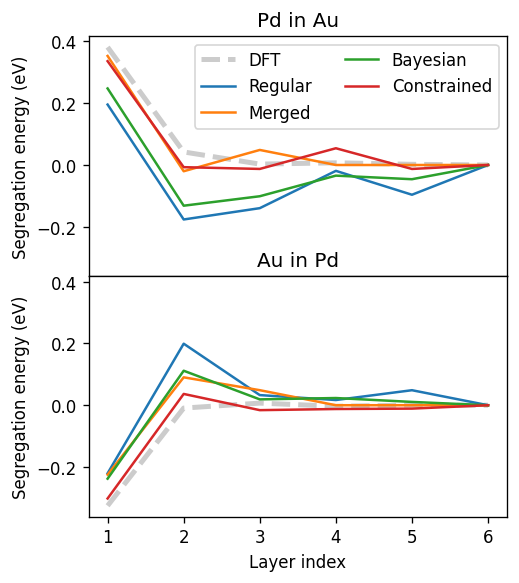
Clearly, the regular cluster expansion results in the worst segregation energy predictions followed by the bayesian cluster expansion, then the merged cluster expansion and lastly the constrained cluster expansion (at the expense of an increased validation error). Note, however, that by tuning the hyperparameters of each approach one would likely be able to change these trends. For instance, in the bayesian approach would approach the merging with sufficiently large coupling.